Introduction
CYPE Sewerage is a program developed for the analysis, design, checking and automatic sizing of sewerage networks in urban infrastructures, or branched sewers, with a single point of discharge and operating by gravity.
The aim in the design of these networks is to evacuate the water from the collection wells to the discharge point. For this purpose, the data and positions of the collection wells and the sewage dump are defined, as well as the layout of the network. In the analysis, the appropriate cross-sections of the sewerage pipes are obtained and it is checked whether the installation complies with the design limitations imposed.
| Note: |
|---|
| Together with other urban infrastructure programs such as CYPE Water Supply and CYPE Gas Supply, other aspects related to the installation design of housing estates can be solved. |
Workflows compatible with the program
As an Open BIM tool connected to the BIMserver.center platform, CYPE Sewerage offers a range of options for your workflow.
Data entry
Open design
- Free network design by manually entering the coordinates of the nodes and drawing the sections that make up the system in CYPE Sewerage.
- Free network design by entering nodes and segments using DXF-DWG or DWF templates, or images (.jpeg, .jpg, .bmp, .wmf) imported into CYPE Sewerage.
Automatic generation of installation geometry from DXF/DWG files
- Import a DXF or DWG file via "Import", "Geometry", and automatically generate the installation geometry based on the information contained within it. This file must use the metre as its drawing unit, and the grid must be close to the coordinate origin. For this option, only the layers containing the sections you wish to use for the generation should be enabled.
Importing data from BIMserver.center
If you link the CYPE Sewerage model to a BIM project on the BIMserver.center platform, you can perform the following actions:
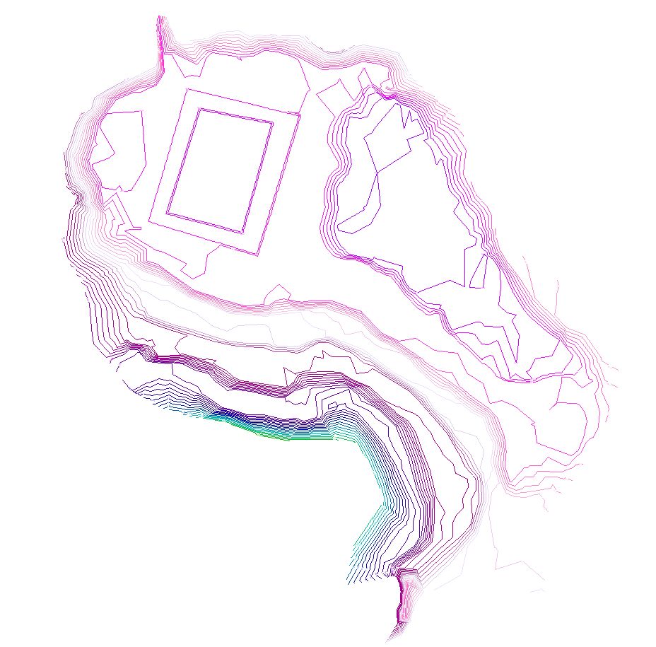
- Importing terrain topography data if the BIM model contains an IFC file with the appropriate features. This allows the topography to be visualised in the 3D view of CYPE Sewerage, displays contour lines in plan view within the general interface workspace, and utilises the imported topography during the data entry process, automatically identifying the elevation values of new nodes entered on it. The available options include the following:
- Importing topographic models in IFC format generated by Open BIM Site.
- Importing topographic models in IFC format generated by other software (such as Aplitop’s TcpMDT applications available on BIMserver.center) and uploaded to the BIMserver.center project via the web platform. The terrain data must be defined as an IfcGeographicElement entity in an IFC4 file.
Data output
- Export reports to HTML, DOCX, PDF, RTF and TXT formats.
- Exporting drawings to DXF, DWG and PDF formats.
- Exporting data generated using CYPE Sewerage to the BIMserver.center platform in IFC and GLTF formats. This enables authorised project stakeholders to view the data.

Work environment
The program has a simple work environment that allows the network design to be carried out quickly by entering and distributing the elements in a single work area on the floor plan.
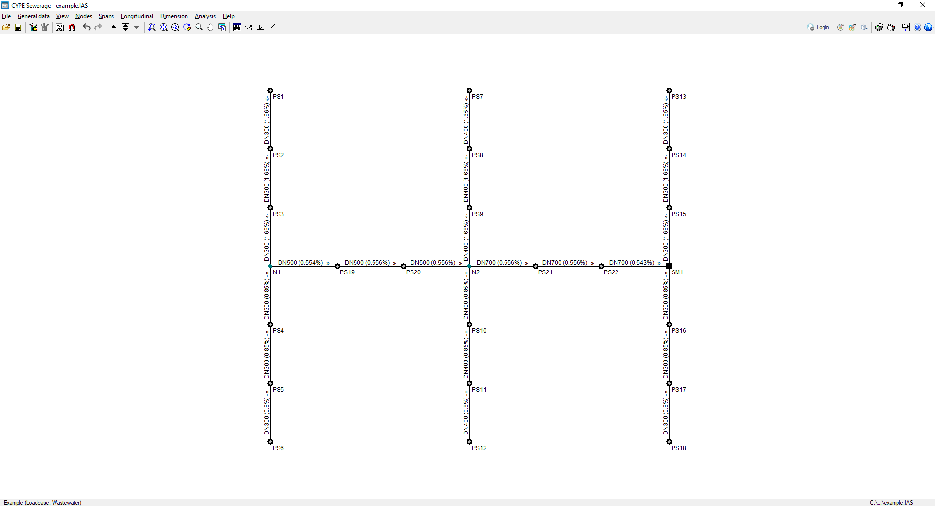
The interface shows the following:
- The menus at the top, where there are tools for:
- accessing the "File" menu;
- configuring the general data;
- controlling the display of the model;
- entering and editing nodes and sections;
- accessing the dimensioning options;
- analysing and designing the network;
- and accessing the "Help" menu.
- The options in these menus also appear in the drop-down options bar, which by default is hidden on the right-hand side.
- An auxiliary horizontal bar, under the menus at the top, where there are tools for:
- accessing the file manager and saving the job;
- accessing the editing resources;
- managing the templates and their snaps;
- undoing and redoing;
- navigating through the different combinations of hypotheses;
- modifying the drawing views;
- viewing the complete drawing map, rotating it, activating orthogonality and controlling the tools for entering by coordinates;
- consulting and managing the connection with BIMserver.center;
- viewing the 3D view of the installation;
- printing the reports and drawings of the job;
- showing or hiding the side drop-down bar of options;
- accessing the available help;
- and accessing the general configuration options.
- Finally, in the central work area, which occupies most of the interface, the elements that make up the network are entered, edited and displayed, as well as the topographic curves, if a model with terrain information has been imported.
Data input and output sequence for designing and analysing sewerage networks
The design and analysis of a sewerage network can be carried out in the program using the following sequence of data input and output:
- Creating a new project (from "File", "New").
- (Optional) Linking to BIMserver.center and importing topographical data from the BIM model.
- Configuring general installation data (in the wizard for creating a new project or via "General data", "Edit general project data"), including the definition of materials and land.
- Defining assumptions and combinations (under "General data", "Edit loadcases"; and under "General data", "Edit combinations").
- (Optional) Importing DXF-DWG/DWF templates or images (from "Edit templates").
- Adding nodes (from "Nodes", "New").
- Adding segments between nodes (from "Segments", "New").
- (Optional) Reviewing and/or adjusting dimensions in the longitudinal sections (from "Longitudinal", "Modify elevations in the longitudinal section").
- Analysing and/or designing the installation (under "Analysis", "Analyse/Design").
- Reviewing the compliance status of the checks performed (via the "Next combination/Select combination/Previous combination" options) and the analysis results (via "Nodes", "Information"; and via "Spans", "Information").
- Printing reports and job drawings (from "File", "Reports/Drawings").
- (Optional) Exporting to BIMserver.center (via "BIMserver.center", "Share").
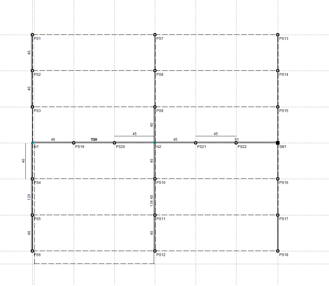
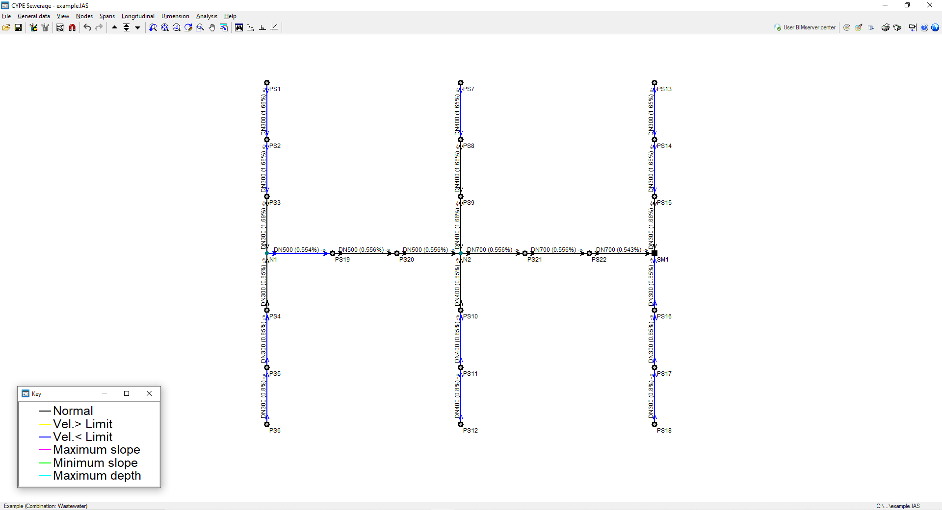
Examples of sewerage networks
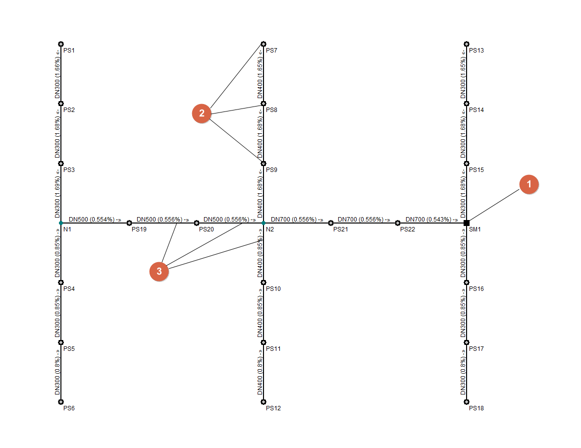
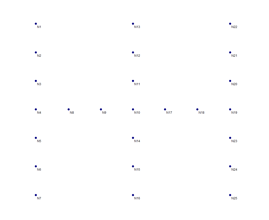
Below is an example of a drainage network that can be created in the program, showing the layout of the components and the options available for adding them to the model:
Combined sewer system for a housing development
- Discharge point or outfall (from "Nodes", "New").
- Sewage or collection wells (from "Nodes", "New").
- Sections (from "Sections", "New").
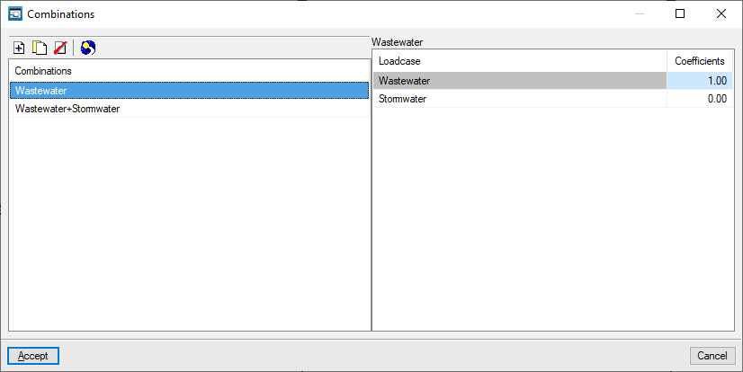
In this case, one loadcase is defined for the discharge of sewage and another for the discharge of rainwater.
In addition, the following combinations are defined, with the indicated percentage of contributions in each loadcase:
- First combination: 100% sewage
- Second combination: 100% sewage, 100% rainwater
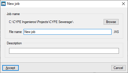
Creating a new job, linking to a project and importing data
When you launch the application and click on "New", you are given the option to create a "New job". After entering the "File name" and "Description", the project can then be added to an existing project on BIMserver.center.
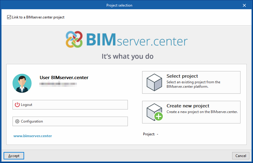
This is done in the "Project selection" window, which offers the following options:
- On the left-hand side, you can log in using a BIMserver.center account.
- On the right-hand side, you will find the "Select project" option to choose an existing project. You also have the option to "Create a new project". In that case, the project you create will be visible on BIMserver.center from that point onwards.
- You have the option to start the project without linking it to the BIMserver.center platform. To do this, simply uncheck the box labelled "Link to a BIMserver.center project", which is located in the top-left corner.
Importing BIM models
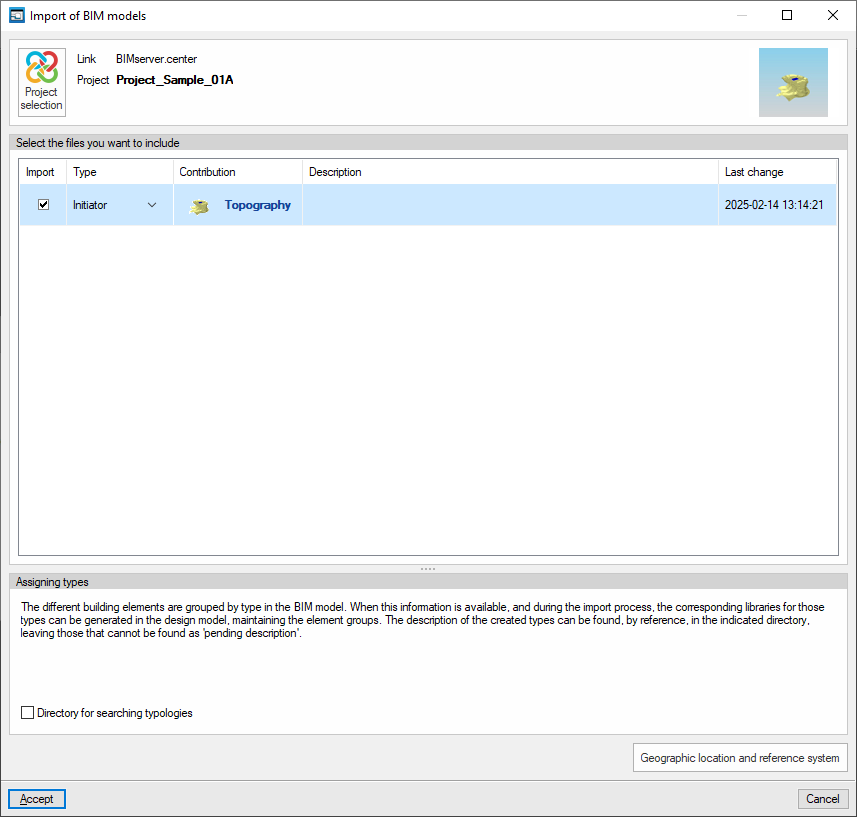
When creating a new project, if you have selected a project hosted on the BIMserver.center platform via "Select project", the "Import BIM models" window will appear, displaying the files contained in that project in IFC format.
To include information from a specific project file, tick the "Import" box and confirm.
Configuring general installation data
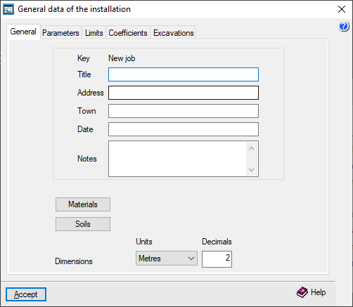
When creating a new project, the program opens the "General installation details" window to ensure that the relevant information is entered, including the definition of materials and plots.
You can access the settings for this data at any time via the "Edit general project details" option in the "General details" menu at the top.
Once you have accepted this window, you will be taken to the program’s main interface.
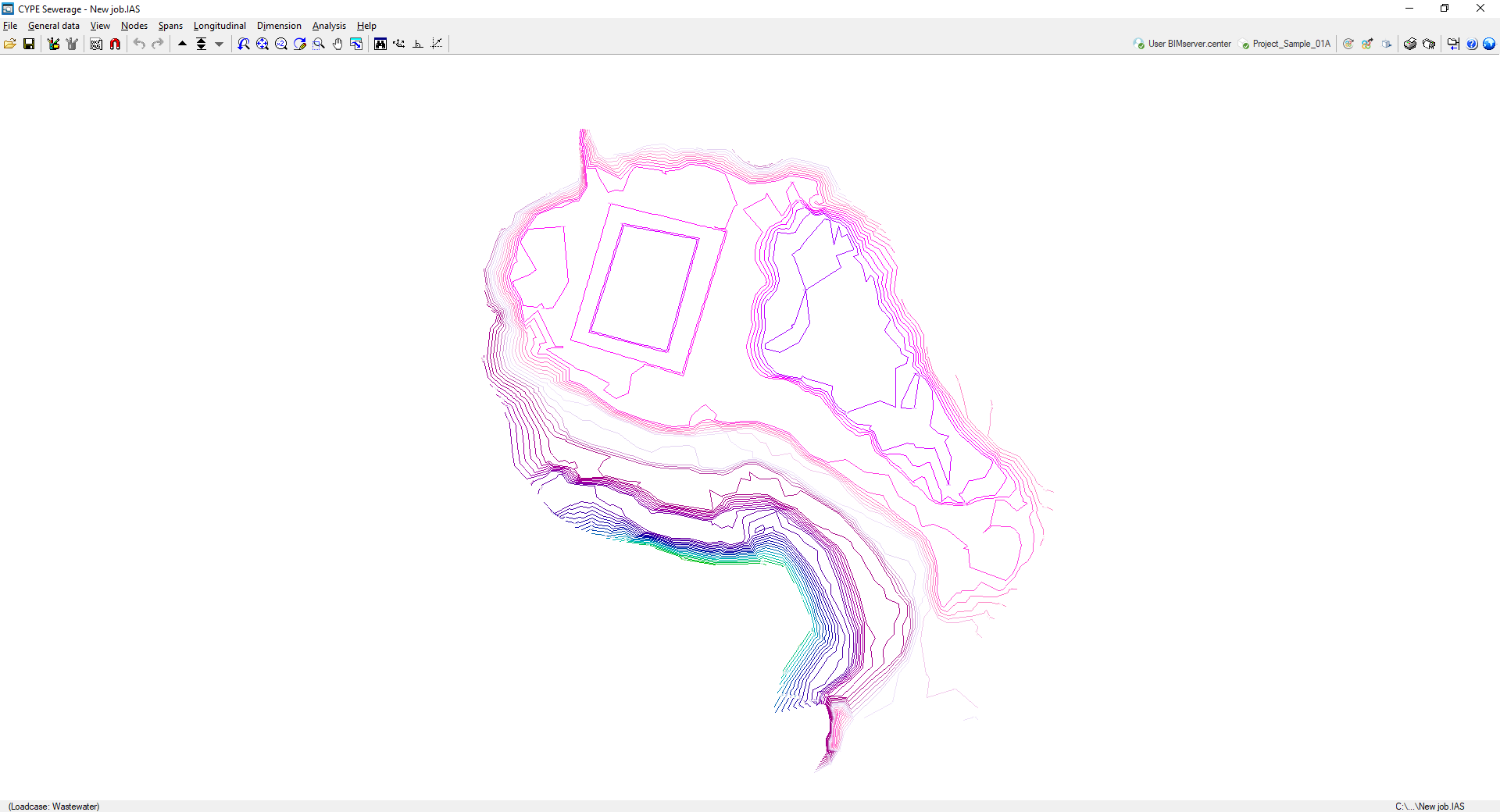
Import results
If an IFC file containing terrain data with the appropriate characteristics has been imported during the creation of a new project, the program will display the contour lines on screen (their visibility can be controlled via the "Show/hide topographic profile lines" option in the "View" menu). When nodes are added, the program will use the elevation data for the terrain at their location.
In addition, the 3D view will display the models included in the BIM project and imported into the job.
Configuring general project data
In the "General data" menu at the top, you will find the "Edit general project data" option, which allows you to enter general information about the installation, such as materials and ground conditions, the parameters, limits and coefficients used in the analysis, and excavation data.

The options available are as follows:
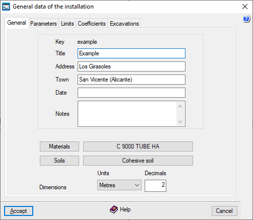
"General" tab
This allows you to enter the following general details, which will appear in the design reports, within the installation description:
- Key
Name of the job. To change it, select "File", then "Save as". - Title
- Address
- Town
- Date
- Notes
In addition, the following options are available:
- Materials
Allows you to manage the materials. - Soils
Allows you to manage the soils. - Settings
for the "Units" and the number of "Decimals" used.
Materials management
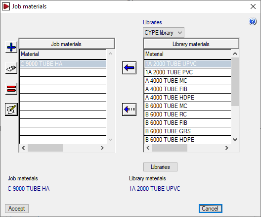
By clicking on the "Materials" button, you can manage the materials used in the site’s pipework, as well as the available material libraries. The window that appears displays two lists:
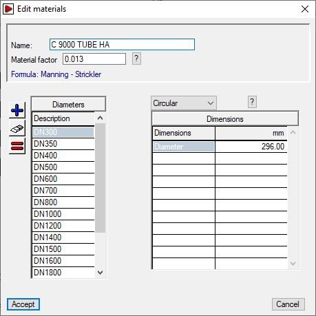
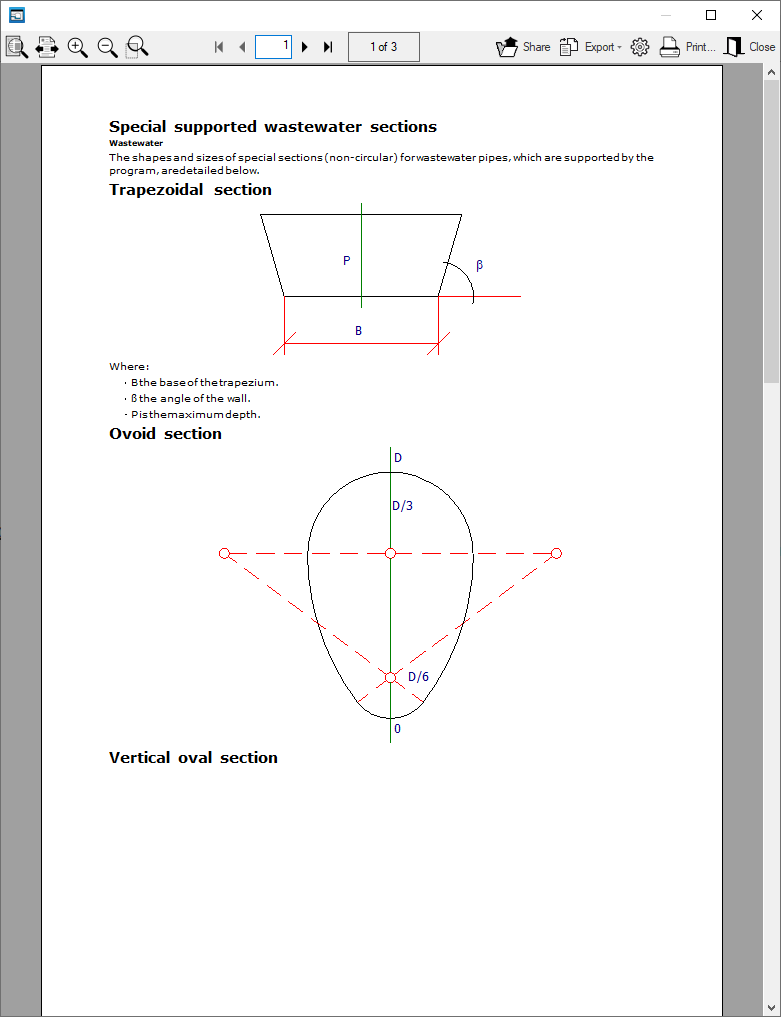
- The list on the left shows the "Job materials". You can create a material manually using the tools on the left or import it from the library materials. When adding or editing a project material, the "Name" and "Material Factor" are specified based on the selected formulation.
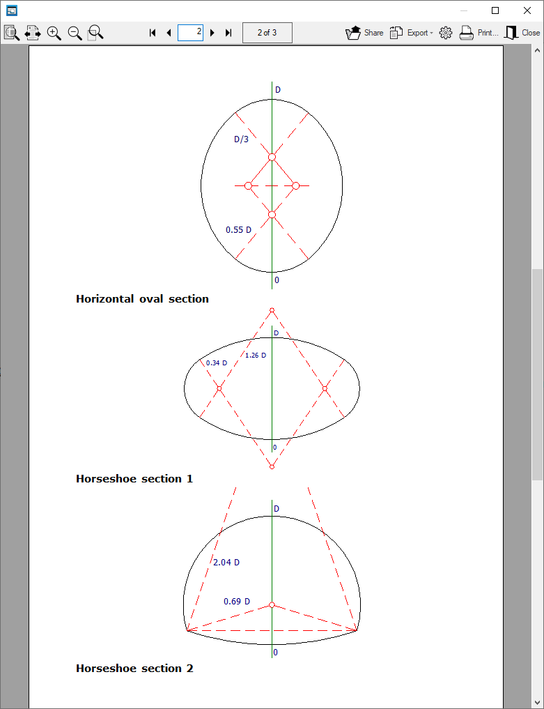
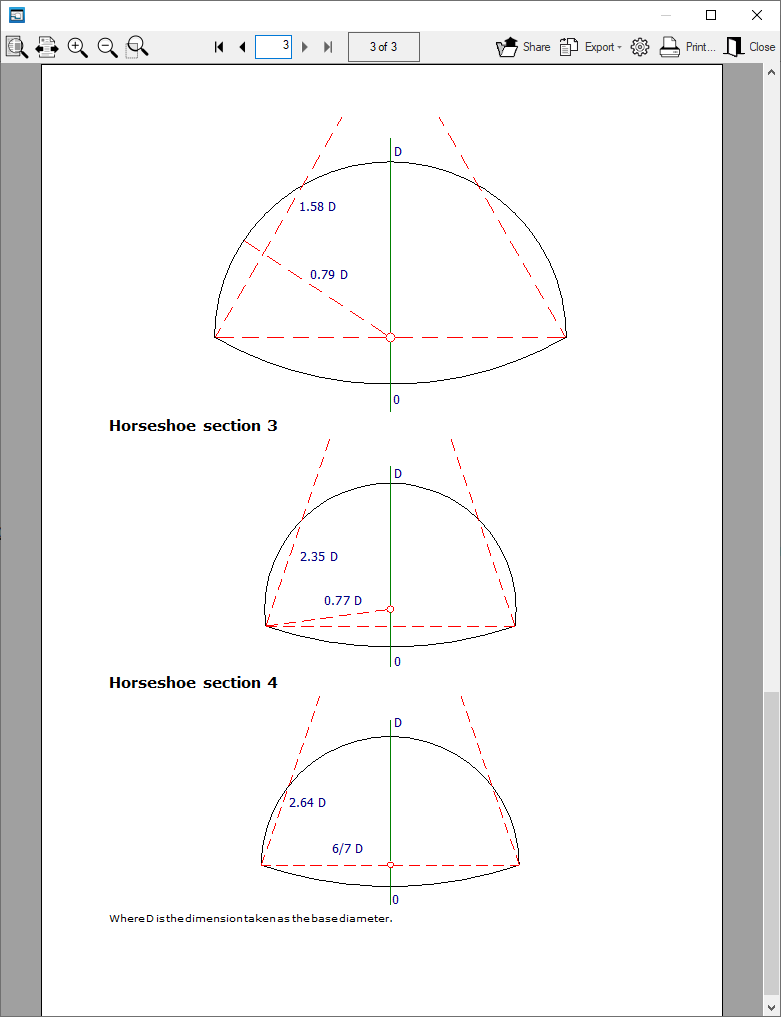
Further down, the “Diameters” table lists the section references associated with the material. On the right, for each section in the list, the section type is selected from the drop-down menu, and the values for its “Dimensions” are detailed, which will depend on the selected section type. The available section types include the following:- Circular, Trapezoidal, Ovoid, Vertical oval, Horizontal oval, Horseshoe
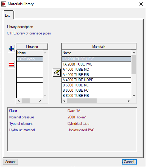
- The list on the right shows the "Library materials". At the top, you can select the library you wish to view. The program includes a default library. You can view the internal data for each library by clicking on the "Libraries" button at the bottom; there, you can define the "Library description" and its "Abbreviation", and for each material included, the "Name" and "Material factor" are displayed based on the selected formulation, as well as the associated section lists.
The first button between the two lists allows you to create a site material by importing information from one of the materials available in the library. The second button allows you to add the grades of the selected library material (on the right) to the selected job material (on the left).
Soils management
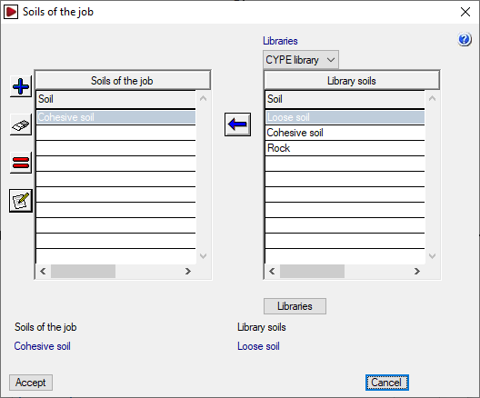
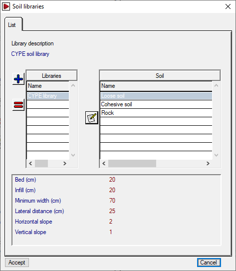
By clicking on the "Soils" button, you can manage the terrains for the project, as well as the available terrain libraries. The window that appears displays two lists:
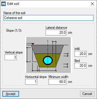
- The list on the left shows the "Site Terrains". You can create a terrain manually using the tools on the left, or import one from the library terrains. When adding or editing a soil in the job, the “Soil name” and the following geometric parameters are specified: “Lateral distance”, “Infill”, “Bed”, “Minimum width”, “Vertical slope” and “Horizontal slope” (which form the “Slope” ratio shown next to the graph).
- The list on the right shows the "Library soils". At the top, you can select the library you wish to display. The program includes a default library. You can view the internal data for each library by clicking on the "Libraries" button at the bottom; there, you can define the "Library description", and its "Abbreviation", and for each plot included, the "Plot name" and the aforementioned geometric parameters are displayed.
The first button between the two lists allows you to create a soil in the job by importing information from one of the soils available in the library. The second button allows you to add the sections of the soils selected from the library on the right to the job soil selected on the left.
To continue creating a new job, you must create at least one material and one soil.
The materials and sites will be available when editing each section via "Spans", "Edit design data".
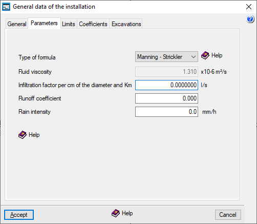
"Parameters" tab
This allows you to define the following design parameters:
- Type of formula
Allows you to select the formulation used to calculate the sections of the sewerage network from the following:- Manning – Strickler
- Prandtl – Colebrook
- Tadini
- Bazin
- Sonier
- Kutter
- Ganguillet - Kutter
- Fluid viscosity
Kinematic viscosity of the fluid; by default, the value 1.31 × 10⁻⁶ m²/s is displayed (1 m²/s = 10,000 Stokes). - Infiltration factor per centimetre of the diameter and kilometre (in l/s)
This factor defines linear inflows into pipelines due to porosity, whether natural, caused by poor maintenance, or intentional. It is defined at a general level and applies to all sections of the project. If you wish to apply it specifically to a particular section, use the corresponding option in the "Sanitation" tab of the "Section edit" window (under "Sections", "Edit design data").
A value can be estimated between 0.0058 l/s = 0.5 m³/day (for new pipes) and 0.0463 l/s = 4 m³/day (for poorly maintained pipes). - Runoff coefficient: A
value of 0.95 may be used for pedestrian areas, roads and plots, and a value of 0.50 for green spaces. - Rain intensity
The maximum rainfall intensity expected for a given return period, corresponding to a rainfall event of a duration equal to the concentration time.
| Note: |
|---|
| The values for "Runoff coefficient" (C, between 0 and 1) and "Rain intensity" (I, in mm/h) entered here will appear in the "Node editing" window for new nodes (as data in the "Contribution" column, if “Rain” loads are selected) and, together with the catchment area (S, in m²), allow the rainwater flow rate (Q, in m³/h) to be calculated using the expression Q=C*I*S/1000. |
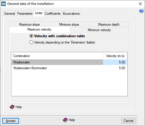
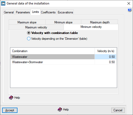
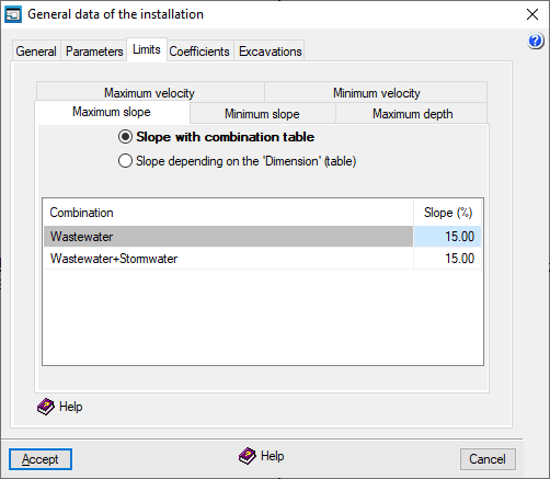
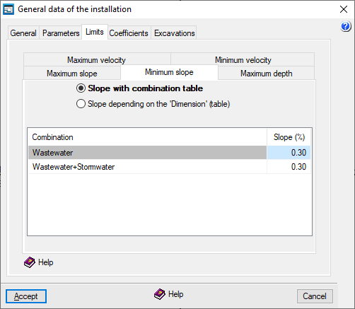
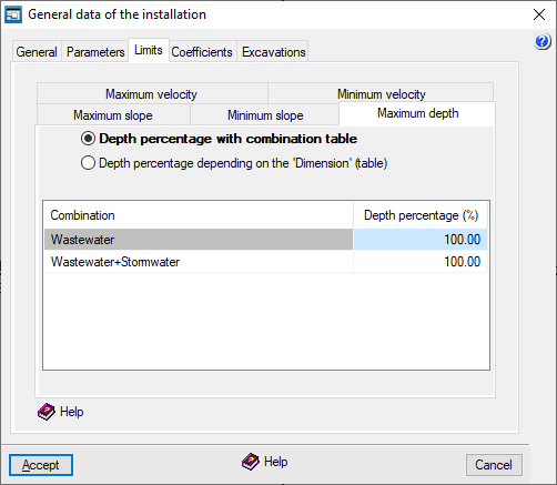
"Limits" tab
This tab allows you to set speed, gradient and draught limits for sections of the installation. These limits operate in two ways:
- If you select the "Analyse" option from the "Analysis" menu, a warning is displayed for those elements of the installation that fall below the minimum values or exceed the maximum values.
- If the "Design" option in the "Analysis" menu is used, the program restricts the system's operation to values within the defined minimum and maximum limits, where possible, as design limits.
The various tabs are used to define the "Maximum speed", "Minimum speed", "Maximum gradient", "Minimum gradient" and "Maximum draught" for the sections.
This can be done:
- By combination table
For each entry, the speed limit, gradient limit or gradient percentage is defined for each combination specified under "General data", "Edit combinations". - Based on "Dimension" (table)
For each entry, the speed limit, gradient limit or draught percentage is defined, which applies to pipelines with dimensions equal to or smaller than those specified. For dimensions larger than those specified, the limit for the largest dimension in the table applies.
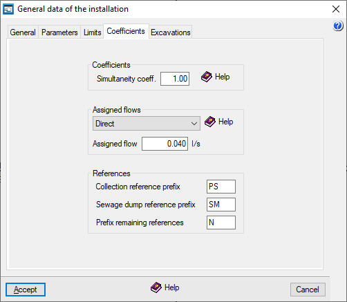
"Coefficients" tab
Coefficients
This allows you to set the following coefficient, which is applied across the board to all analyses for the project:
- Simultaneity coefficient
This allows you to increase or decrease the inflows into the collection wells. It is defined as a ratio of one and is applied to the wells in all combinations. This makes it possible to simulate operations at different times of the day or seasonal changes. By default, a value of one is set.
Assigned flows
This allows you to specify whether the loads for collection wells are defined by default directly or by allocation.
- Direct
The discharge will be fed directly into the flow units. - Per allocation
The discharge will be calculated based on the flow rate per allocation (which corresponds to the value entered in the "Allocation" field) and the corresponding number of units.
The load values and their definition type can be edited later in the edit panel for each node.
References
This allows you to set the prefixes that are automatically added to the references of the installation nodes when they are added to the workspace, whether they are collection wells, discharge points or other nodes:
- Collection reference prefix
- Sewage dump reference prefix
- Remaining reference prefix
References can be edited later in the edit panel for each node.
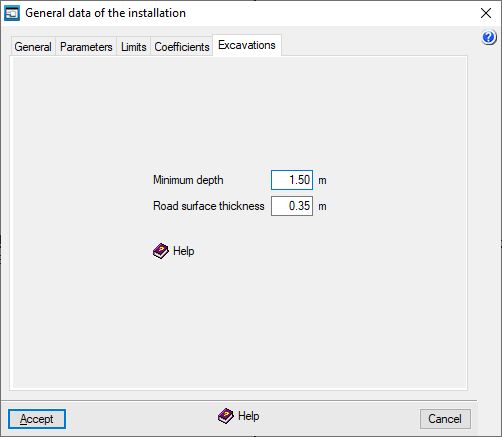
"Excavations" tab
This tab allows you to define the following parameters relating to the site's excavations:
- Minimum depth
Allows you to set an alarm that alerts you when any point in the installation falls below this value (in the "Analysis results" report that appears after using the options in the "Analysis" menu). The minimum depth is measured from the ground level to the top edge of the inner face of the duct. - Road surface thickness
This indicates the default distance between the road surface and the modified ground level. By default, this value is subtracted from the road surface elevation (entered in the "Edit node" panel) to obtain the ground level without the need to enter it manually. Furthermore, if the ground level is changed in that panel, a warning will be displayed if the specified road surface thickness is not met.
| Note: |
|---|
| Where there are multiple road surface thicknesses in the project, if the "Road surface thickness" value is changed in this section, any new nodes added from this point onwards will be analysed using the new thickness, but the previous thickness will be retained for nodes added earlier. |
Defining loadcases and combinations
The "General data" menu at the top contains the following options, which allow you to define the project’s loadcases and combinations:

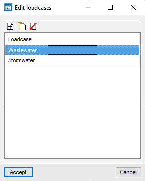
Edit loadcases
This allows you to define the basic parameters of the installation.
To do this, add elements to the list and type in their names.
Once the loadcases have been defined, contributions can be assigned to each of them via the "Nodes", "Edit design data" option. The coefficients corresponding to the laodcase combinations must also be defined via the "General data", "Edit combinations" option.
Edit combinations
This allows you to define combinations of loadcases.
To do this, items are added to the left-hand list, and their names are entered. Then, in the right-hand list, the combination coefficients (expressed as fractions) assigned to each loadcase in the selected combination are indicated.
The loadcases must have been entered previously via "General data", "Edit loadcase".
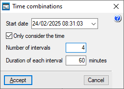
The program also includes a feature for automatically creating "Time combinations" by specifying a particular "Number of intervals" and the "Duration of each interval" from a "Start date". If you select the "Only consider time" option, only the time—and not the date—is included in the reference for the generated combinations.
Options in the "View" menu
From the "View" menu at the top of the interface, you can access the following options:

View configuration
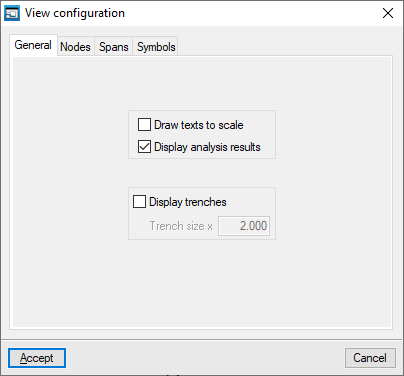
This allows you to control how the diagram elements are displayed on screen. The available options are as follows:
- "General" tab
- Draw text to scale (optional)
- Display analysis results (optional)
- Display trenches (optional)
- Trench size x (value)
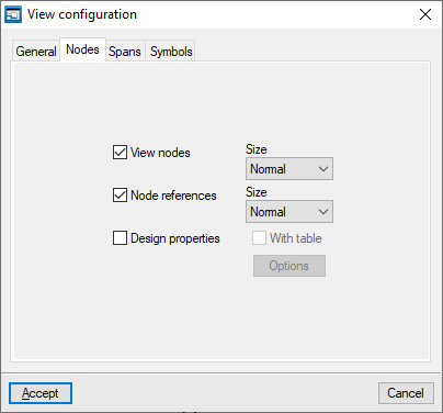
- "Nodes" tab
- View nodes (optional)
- Node reference (optional)
- Design properties
- Options: Data to display on nodes
- With table (optional)
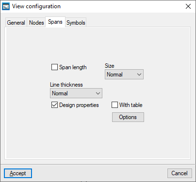
- "Spans" tab
- Span length (optional)
- Line thickness
- Design properties (optional)
- Options: Data to be displayed by section
- With table (optional)
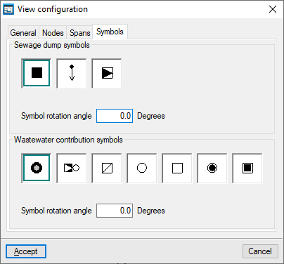
- "Symbols" tab
- Sewage dump symbols
- Rotation angle symbol
- Wastewater contribution symbol
- Rotation angle symbol
- Sewage dump symbols
Show/hide the contour lines
This allows you to show or hide the contour lines generated on screen if you have imported an IFC file containing the terrain model during the project creation process.
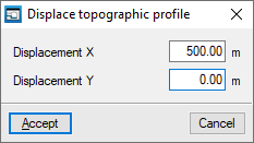
Displace topographic profile
This allows you to reposition the generated topographic profile if you have imported an IFC file containing the terrain model during the project creation process.
Entering and editing nodes
The "Nodes" menu at the top of the program interface contains the following options for creating and editing installation nodes:
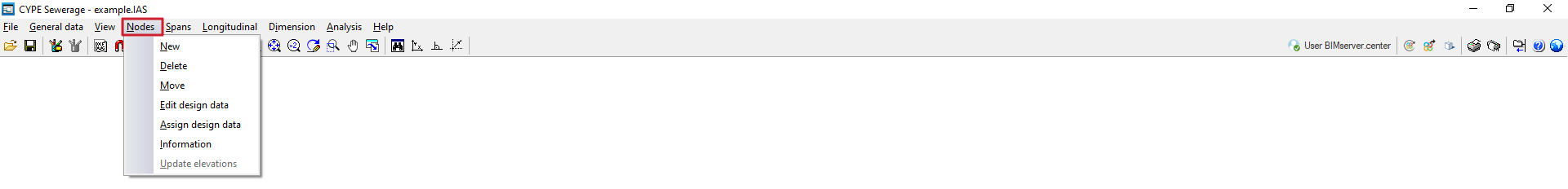
New
Allows you to insert nodes in the workspace.
Nodes are created by default as transition nodes, i.e. nodes without loads that allow changes in direction whilst maintaining the continuity of the section in the dimensioning. They can subsequently be edited via "Nodes", "Edit design data". If you right-click when entering a new node, you can also access the design data editing panel for the node being entered.
There are several ways to position the nodes on the model when using this option:
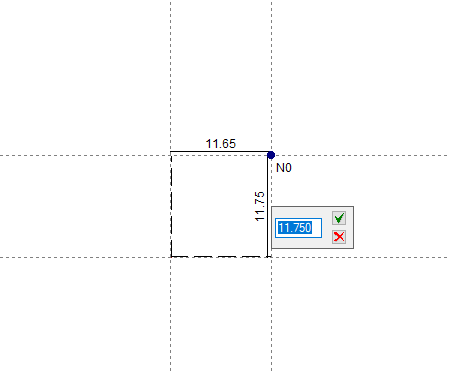
- By absolute coordinates
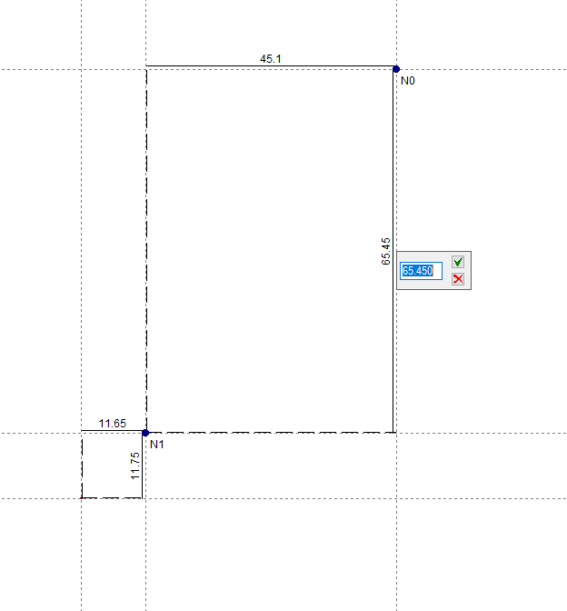
When entering the first node or base node of the installation by left-clicking on the screen, enter the node’s absolute X-coordinate and press "Enter"; then enter the absolute Y-coordinate and press "Enter" again. - By relative coordinates:
A base node has been entered; the remaining nodes can be added using relative coordinates, i.e. by specifying distances relative to other nodes. To do this, left-click on the screen where you wish to insert the node and enter the relative X and Y coordinates relative to the position of the nearest node. - Importing DXF or DWG files
The options for importing DXF or DWG files can be used to add nodes and segments. - Automatic geometry generation
Under the "File" menu, select "Import" and then "Geometry" to automatically generate the installation geometry from a DXF or DWG file. This file must use the metre as its drawing unit, and the network must be close to the coordinate origin. In this option, you should only activate the layers containing the sections you wish to use for the generation.
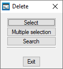
Delete
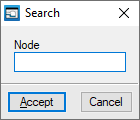
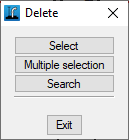
This allows you to delete the selected node. You can use the left mouse button to draw a rectangular selection area on the screen to delete multiple nodes. Furthermore, clicking the right mouse button brings up options to "Select" a single node, perform a "Multiple selection" node by node, or "Search" for a node by its reference.
Move
This allows you to reposition the selected node. After clicking on the node, click on another point to specify the new position.
Edit analysis data
This allows you to edit the selected node. You can use the left mouse button to draw a rectangular selection area on the screen to edit multiple nodes, selecting the fields you wish to edit. Furthermore, clicking the right mouse button brings up options to "Select" a single node, perform a "Multiple selection" node by node, or "Search" for a node by its reference.
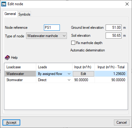
In the edit window that appears, enter the node details:
- "General" tab
- Node reference
- Type of node
- Wastewater manhole
A node where a collected water flow rate is defined for each loadcase. When this type of node is selected, the program displays a table at the bottom that allows you to define the inflow rate for each loadcase. This table contains the following columns:- Loadcase
- Loads
The load can be defined in various ways:- Direct
- By allocation
- Rainwater
- Input
The inflow rate is defined by entering its value directly if the "Direct" option has been selected; by entering a value for “Allocation” and the “Number of units” to be considered, if the “By allocation” option has been selected; or by defining the “Runoff coefficient”, the “Slope area” and the “Rainfall intensity”, if the “Rainfall” option has been selected. - Total input
Displays the total inflow rate.
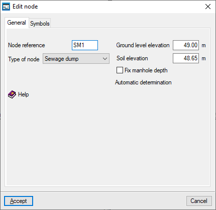
- Sewage dump
The facility’s discharge point. A single discharge point must be defined for the network. This point may represent a pumping station, an outfall or an existing sewerage network. - Transition node
A node without any additional material that allows changes in direction whilst maintaining the continuity of the section in the design.
- Wastewater manhole
- Ground level elevation
The level reached by the surface after the trenches have been backfilled and the road surface has been laid. - Soil elevation
The level of the modified ground (not the undisturbed ground) from which excavation begins. The difference between the finished ground level and the ground level must be greater than the value for "Road surface thickness" defined under "General data", "Edit general project data". - Fix manhole depth (optional)
If this option remains disabled, the program automatically determines the manhole depth as the greatest depth of the intersecting sections. If enabled, you can enter the manhole depth.
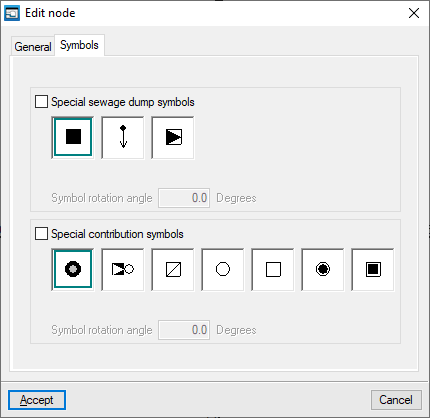
- "Symbols" tab
Allows you to define specific symbols for the node being edited.- Specific sewage dump symbols (optional)
- Specific contribution symbols (optional)
Assign analysis data
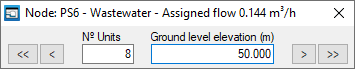
It allows you to assign data to nodes quickly.
When you click on the option, a small window opens in the top-left corner of the screen. At the same time, the node with the lowest reference number will be highlighted in yellow, and you can view and/or edit the node’s data (such as the number of units, flow rate and grade line). You can navigate through all the nodes using the relevant buttons.
Information
This allows you to view the data entered in the node.
If the structure has been analysed, the analysis results for the node under the currently selected loadcase are also displayed. Furthermore, clicking on the node opens a window where you can view the results for any load, loadcase, envelope and oscillation, both analytically and graphically: the "Graphs" button displays the "Flow rate" graph for the different load cases.
Update dimensions
Update the elevations of all nodes based on the terrain topography defined in the BIM model.
Entering and editing spans
The "Spans" menu at the top of the program interface contains the following options for entering and editing installation spans:
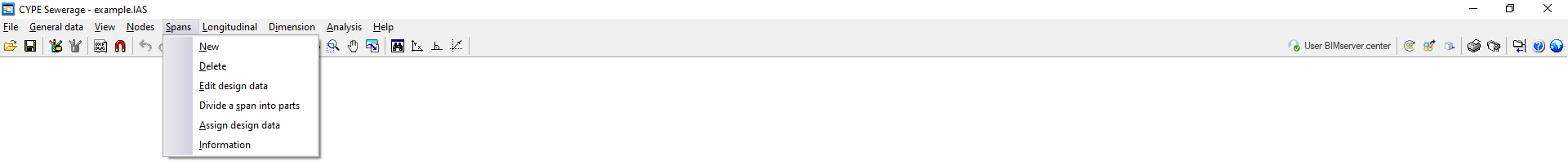
New
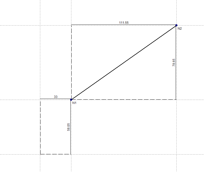
This allows you to insert a new span into the workspace. This can be done:
- By selecting two previously created nodes from "Nodes", "New".
- Or by simply selecting two points on the workspace, which will define the end nodes of the span. This means there is no need to enter the nodes defining the span beforehand. When doing this, you must specify the absolute or relative coordinates of each node or capture points from a template, just as you would when adding new nodes.
In addition, the following is taken into account:
- If, when creating a new span, it crosses an existing span, a new node will be created at that intersection.
- If, when you insert a span, the mouse pointer is positioned over the centre of a node, the end of the span will be that node. Otherwise, a new node will be created at that point.
- You can also click on a previously entered span to start from that point and create a node at the desired location.
The end nodes of the inserted spans are created by default as transition nodes; that is, nodes without load input that allow changes in direction whilst maintaining the span’s continuity in the analysis. They can subsequently be edited via “Nodes”, “Edit design data”.
| Note: |
|---|
| The installation must be interconnected; in other words, all nodes entered in the project must be connected by spans belonging to the same network with a single discharge point. It is not possible to include two separate networks in the same file. |
Delete
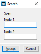
This allows you to delete the selected span. You can use the left mouse button to draw a rectangular selection area on the screen to delete multiple spans. Furthermore, clicking the right mouse button brings up options to "Select" a single span, perform a "Multiple selection" span by span, or "Search" for a span using the coordinates of its endpoints.
When a span is deleted, the end nodes are also removed if they belong solely to the deleted span.
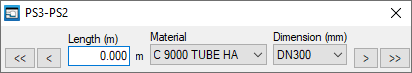
Edit design data
This allows you to edit the selected span. You can use the left mouse button to draw a rectangular selection area on the screen to edit multiple spans, selecting the fields you wish to edit. Furthermore, clicking the right mouse button brings up options to "Select" a single span, perform a "Multiple selection" span by span, or "Search" for a span using the coordinates of its end nodes.
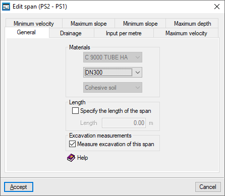
In the edit window that appears, enter the details of the span:
- "General" tab
- Materials
- Span material
Determines the range of diameters available for the span, both for manual selection and for preliminary design. In the latter case, the program will attempt to find a diameter that meets the requirements without changing the span material. - Pipe diameter
This determines the main design parameters for the pipe span. During preliminary sizing, the diameter that best fits the existing network is selected from among those defined for the material chosen for the pipe span. - Span terrain
The terrain where the trench through which the span runs is excavated. This parameter does not appear if no terrain has been selected for the project.
- Span material
- Length
The program allows you to determine the length of the span based on the drawing provided or to enter the value directly. In the first case, the "Specify span length" checkbox remains unchecked, and the length of the span is calculated based on the coordinates of the end nodes (including their elevation). In the second case, the "Specify the length of the span" checkbox is enabled, and the length value used to analyse that span is entered. This option allows you to enter diagrams that do not need to be drawn to scale.- Specify the length of the span (optional)
- excavation survey
- Measure excavation of this span (optional)
- Materials
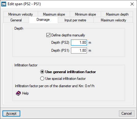
- "Drainage" tab
- Depth
- Set depths manually (optional)
When this box is ticked, the program allows you to set the depth of the duct at the end nodes of the span, measured from the ground level at the nodes to the lower edge of the inner surface of the duct.
- Set depths manually (optional)
- Infiltration factor
- Use general infiltration factor
If this option is selected, the program will use the infiltration factor defined for the entire project under "General data", "Edit general project data". - Use specific infiltration factor
If this option is selected, you must define the infiltration factor per centimetre of diameter and per kilometre for the span being edited.
- Use general infiltration factor
- Depth
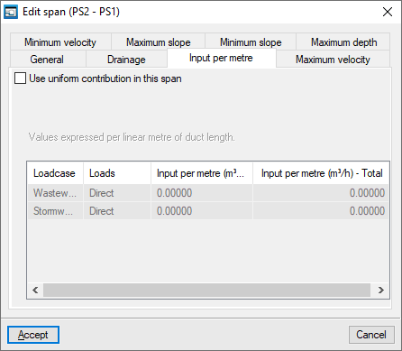
- "Inflow per metre" tab
This allows you to define a uniform inflow rate for the span. The values are expressed per linear metre of pipeline length.- Use uniform contribution this span (optional)
When this box is ticked, the program displays a table at the bottom that allows you to define the inflow rate for each loadcase. This table contains the following columns:- Loadcase
- Loads
The load can be defined in two ways:- Direct
- By allocation
- Rainwater
- Inflow per metre
The inflow rate per linear metre is defined by entering its value directly if the "Direct" option has been selected; by entering a value for “Allocation” and the “Number of units” to be considered, if the “By allocation” option has been selected; or by defining the “Runoff coefficient”, the “Slope area” and the “Rainfall intensity”, if the “Rainfall” option has been selected. - Total inflow per metre
Displays the total inflow rate per linear metre of pipeline.
- Use uniform contribution this span (optional)
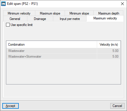
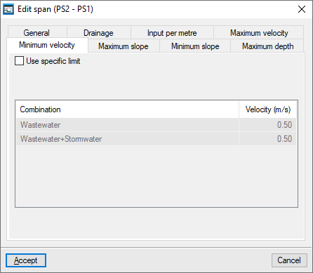
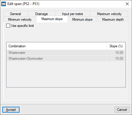
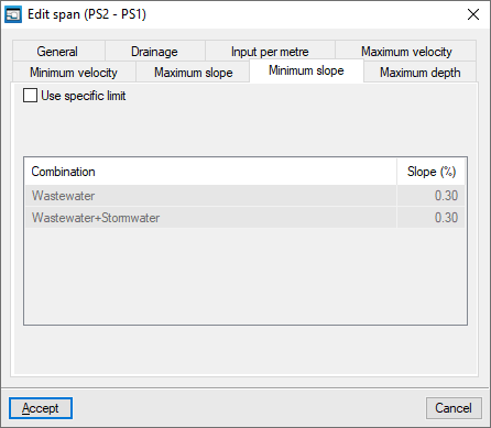
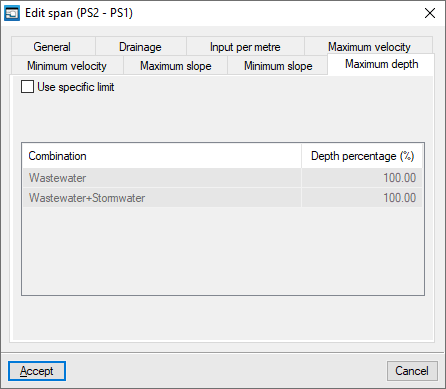
- The "Maximum velocity", "Minimum velocity", "Maximum slope", "Minimum slope" and "Maximum depth" tabs
These tabs allow you to enter specific limits for velocity, slope and depth percentage for the span being edited, for each of the loadcase combinations shown in the table.- Use custom limit (optional)
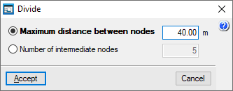
Divide a span into parts
This allows you to select a span and split it into several spans, automatically creating nodes along the span. This can be done by specifying the "Maximum distance between nodes" or the "Number of intermediate nodes".
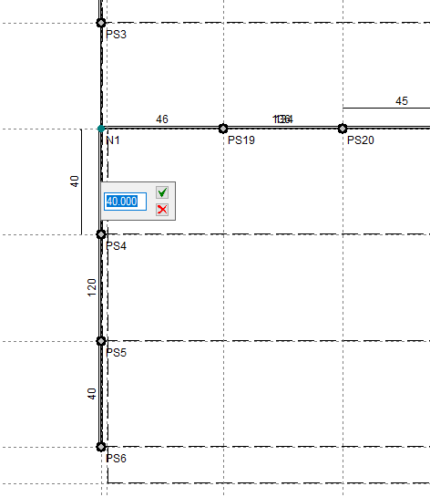
Assign design data
It allows you to quickly assign data to spans.
When you click on the option, a small window opens in the top-left corner of the screen. At the same time, the selected span will be highlighted in yellow; initially, the one with the lowest node references. You can review and/or modify the span’s details (such as length, material and dimensions). You can navigate through all the spans using the relevant buttons.
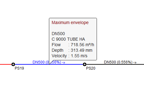
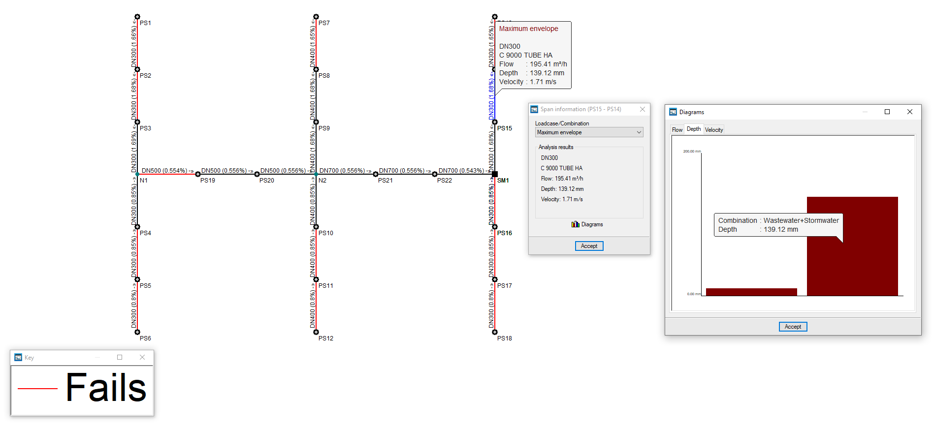
Information
This allows you to view the data entered in the span.
If the job has been analysed, the analysis results for the span under the currently selected loadcase are also displayed. Furthermore, clicking on the span will open a window where you can view the results for any loadcase, combination, envelope and oscillation, both analytically and graphically. The "Graphs" button displays the "Flow", "Depth" and "Velocity" graphs for the different combinations.
Editing longitudinal sections
In the "Longitudinal" menu at the top of the program interface, you will find the following option:

Modify dimensions in the longitudinal section
This allows you to modify the elevation levels of the installation graphically, displaying the longitudinal section of the selected spans.
To use this option, you must have entered the geometry of the network spans on the plan view and assigned the discharge point. Clicking a span opens a window showing the span's longitudinal section and the spans that follow it up to the discharge point.
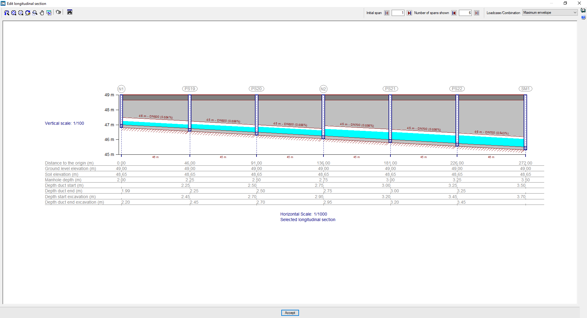
In the longitudinal section view, you can configure the "Initial span" and the "Number of spans displayed" up to the discharge point you wish to view using the options at the top. By default, the first section to be displayed will be the one marked on the plan view in the main interface, and the subsequent sections will show the route to the discharge point.
In the "Loadcase/Combination" selector, you can adjust the display of the water table for different combinations or envelopes.
In the longitudinal section itself, clicking on the sections directly changes the "Slope of the span". When the new slope is set, the program calculates the depth of the manhole located at the end of the modified span.
In addition, the following changes can be made:
- By clicking the scaling options ("Horizontal scale" and "Vertical scale"), you can change the section's horizontal and vertical display scales.
- By clicking on the text at the bottom, you can change the "Longitudinal section name".
In the top-left corner, the program provides tools for printing the "Drawings" associated with the selected longitudinal section (both the site plan showing its position and the longitudinal section plan), as well as for viewing its position on the network via a "Map".
In the information panel at the bottom of the timeline, you can view or edit the following data for each node. The cursor changes when you hover over the data you wish to edit, indicating that it is editable:
- Distance to the origin:
The horizontal distance from the well to the origin of the first span of the longitudinal section shown. - Ground level elevation (editable)
Level of the finished ground level elevation. - Soil elevation (editable)
Modified soil elevation, excluding the thickness of the road surface. - Manhole depth (editable)
The depth of the manhole, measured from ground level. - Depth duct start (editable)
The depth of the lower edge of the inner surface of the inlet duct to the shaft, measured from ground level. - Depth duct end (editable)
Depth of the lower edge of the inner surface of the manhole’s outlet conduit, measured from ground level. - Depth start excavation
The depth of the excavated ground at the entrance to the shaft, measured from the ground level elevation. - Depth duct end excavation
The depth of the excavated ground at the well outlet, measured from the ground level elevation.
Dimensioning options
The "Dimension" menu at the top of the program interface contains options for modifying and/or displaying the dimensions and reference lines between node alignments, which define the geometry of the installation:

Change the spacing between rows
You can adjust the distance between node alignments by clicking directly on the dimensions displayed on the screen.
Show/hide guide lines
This allows you to show or hide the dimensions in the workspace and the reference lines passing through the nodes.
Analysing, checking and designing
The "Analysis" menu at the top of the program interface contains the options for carrying out the analyses, checks and designs of the installation:

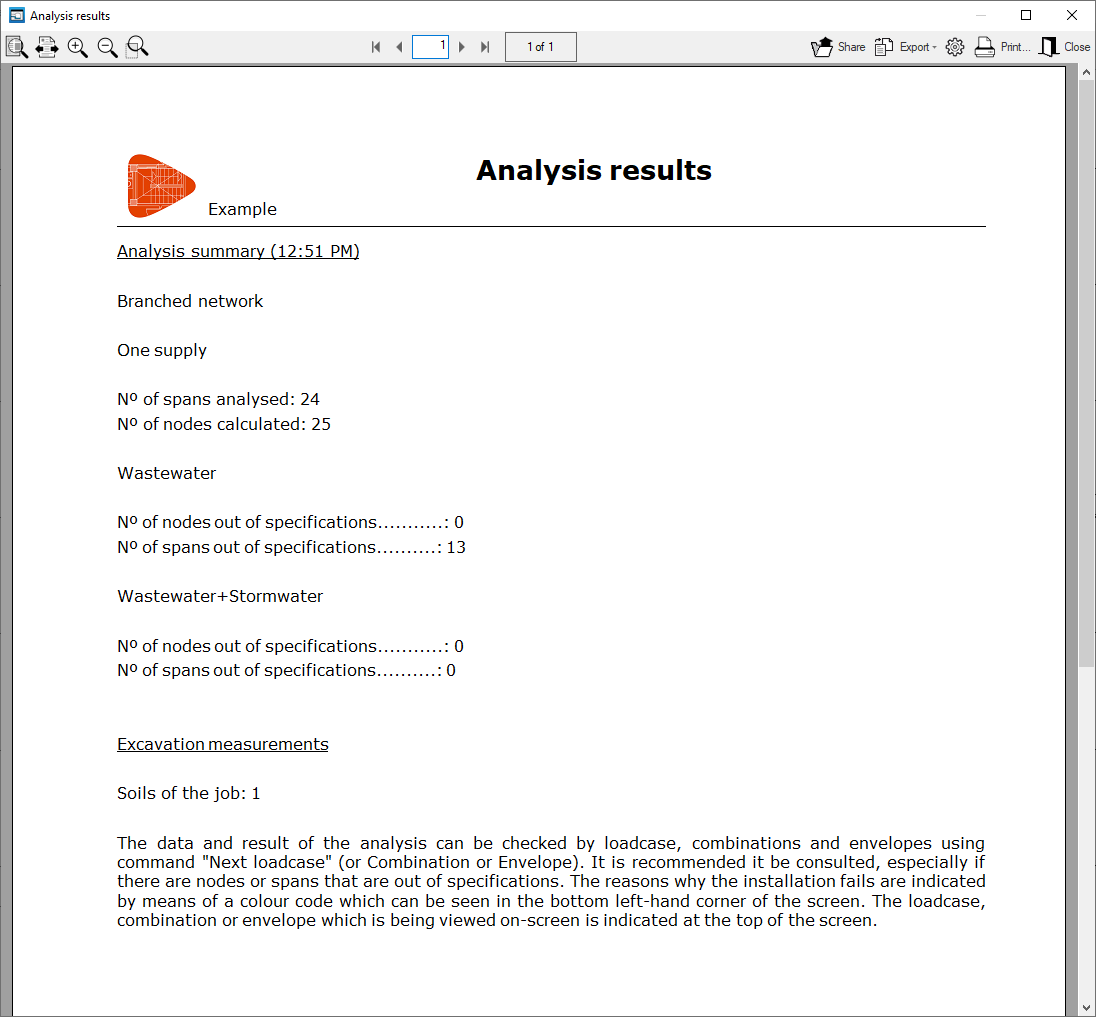
Analysis
This allows you to analyse and check the installation using the data entered.
The program uses a method of calculating flow rates from the inflows at the wells to the outfall. For this reason, the network must be branched and have a single discharge point.
Once the process is complete, a dialogue box appears showing the analysis results.
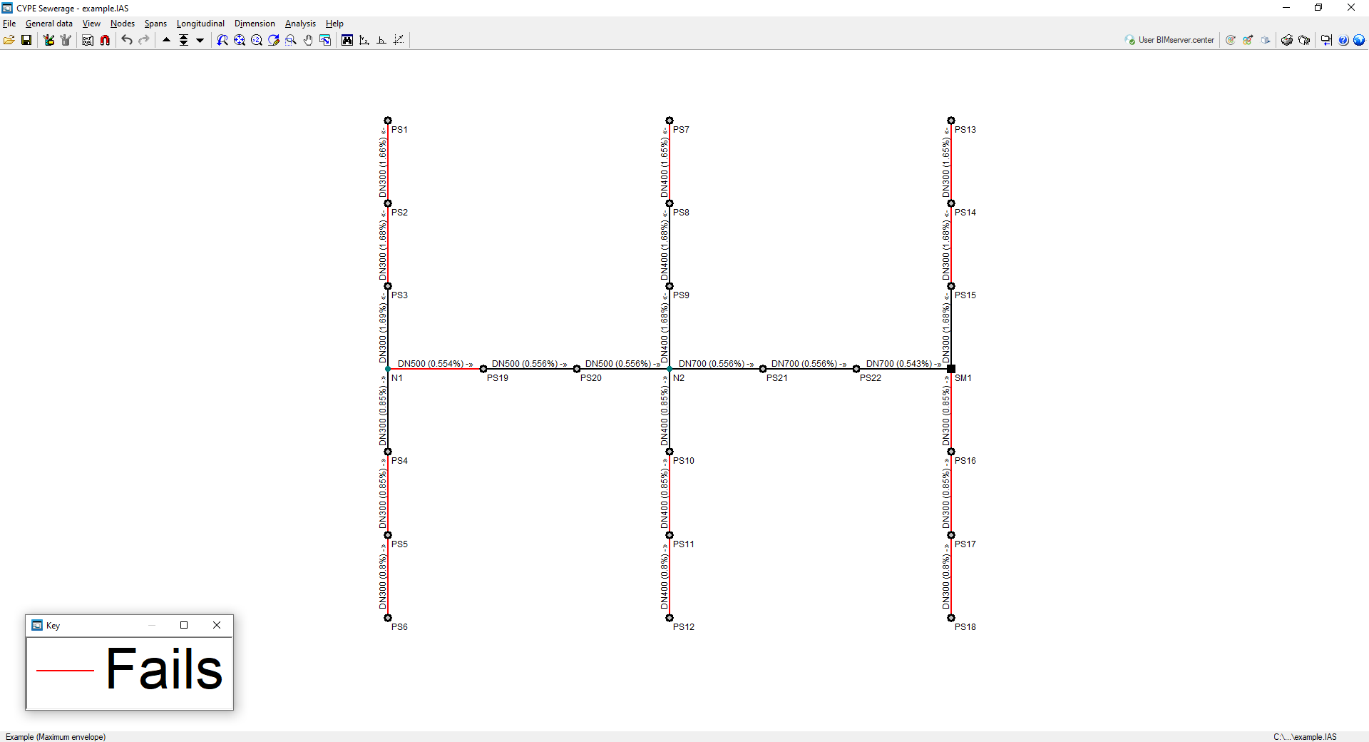
In the workspace, once the analysis has been carried out, any spans that do not meet a particular constraint will be highlighted in red.
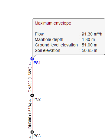
The program will display the "Maximum envelope", the "Minimum envelope" and the "Oscillation", which are added to the list of combinations. The term "envelopes" refers to the highest and lowest values in each section of all the defined combinations. The oscillation is the difference between the highest and lowest value envelopes.
To view the data and results for the various scenarios, combinations and envelopes, use the "Next combination", "Select combination" and "Previous combination" options at the top of the screen. The envelopes will only indicate whether all constraints are met for that span or not.
To find out why a section is non-compliant, you must select a combination and check the colour-coded "Legend" that appears in a separate window. The colour code indicates the reasons why the sections of the installation are non-compliant.
In the bar at the bottom of the interface, the label shows the name of the project and the loadcase, envelope or combination currently being displayed on screen.
Dimension
Launch the automatic preliminary design process for the installation. During the preliminary design, the program will attempt to optimise the design and select the minimum diameter that meets all speed and clearance constraints, whilst maintaining the selected material.
You can then assign the preliminary design results to the project and carry out the analyses.
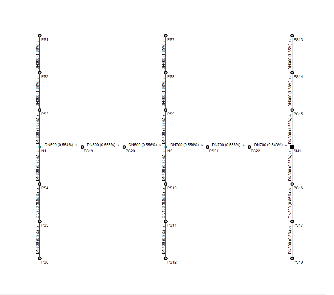
Results output
Viewing results on screen
After the analysis, the program displays the results on the screen when selecting an element of the installation via "Nodes", "Information", or via "Sections", "Information".
This includes the analysis data of the nodes and the analysis data of the sections, with results by laodcases, combinations or envelopes.
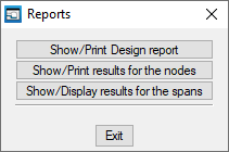
Reports
The program can be used to print the reports directly or to generate HTML, PDF, TXT, RTF or DOCX files.
The reports are obtained via the "Reports" option in the "File" menu or from the right-hand side of the top toolbar.
The following reports are available:
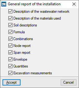
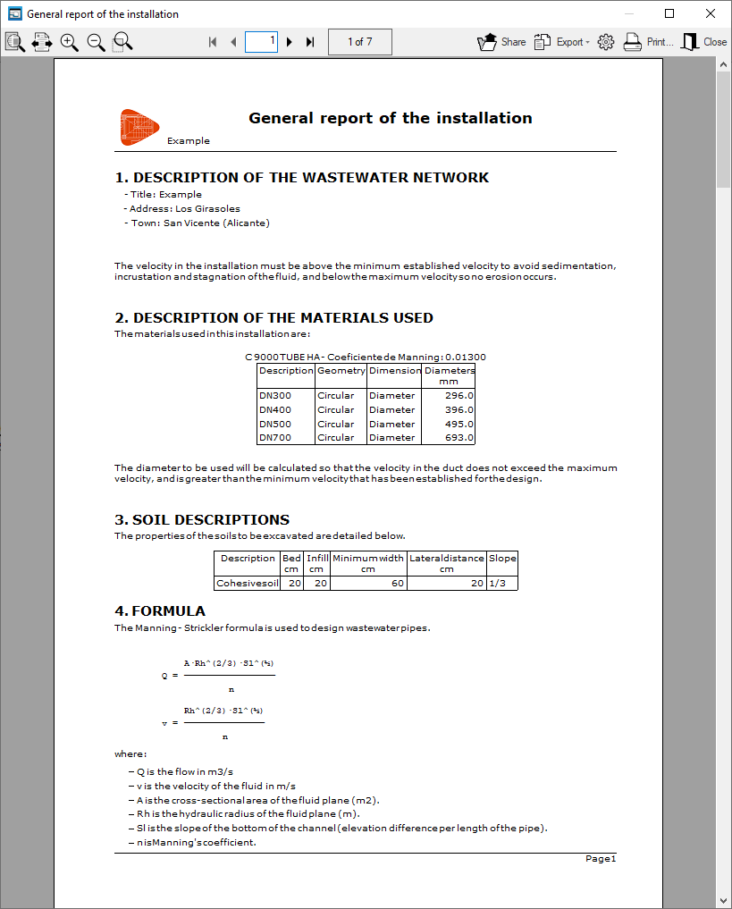
- Calculation report
Prints the general report of the installation. It includes the following sections, which can be activated or deactivated:- Gas network description (optional)
- Description of the materials used (optional)
- Soil descriptions (optional)
- Formula (optional)
- Combinations (optional)
- Node report (optional)
- Span report (optional)
- Envelope (optional)
- Quantities (optional)
- Excavation measurements (optional)
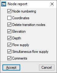
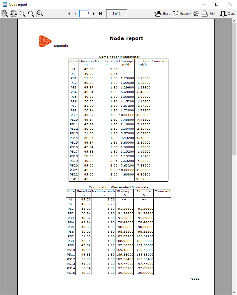
- Node report
Prints the report of the results in the nodes. It includes the following information, which can be activated or deactivated:- Node numbering (optional)
- Coordinates (optional)
- Delete transition nodes (optional)
- Installed flow (optional)
- Required flow (optional)
- Piezometric head (optional)
- Available pressure (optional)
- Comments (optional)
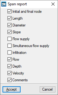
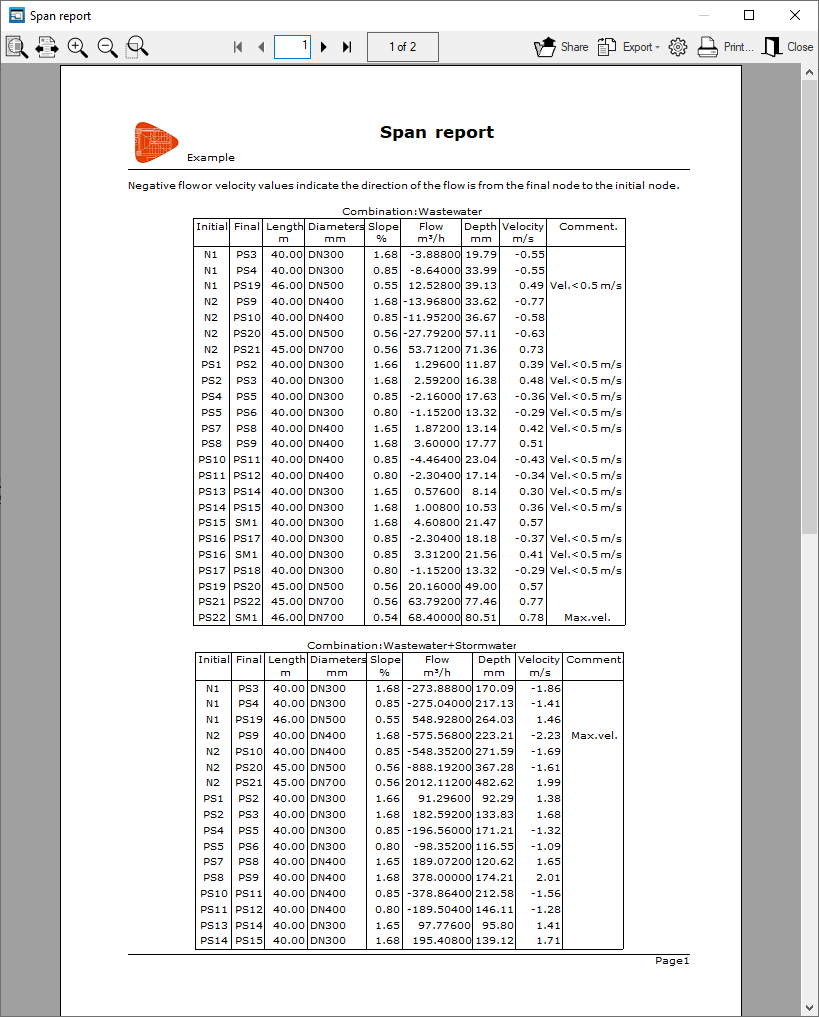
- Span report
Prints the report of the results in the spans. It includes the following information, which can be activated or deactivated:- Initial and final node (optional)
- Length (optional)
- Diameter (optional)
- Installed flow (optional)
- Required flow (optional)
- Flow (optional)
- Velocity (optional)
- Losses (optional)
- Comments (optional)
Drawings
The program can print the job drawings on any graphic peripheral configured on the computer or create DWG, DXF or PDF files.
The drawings are obtained from the "Drawings" option in the "File" menu or from the right-hand side of the top toolbar.
The following drawings are available:
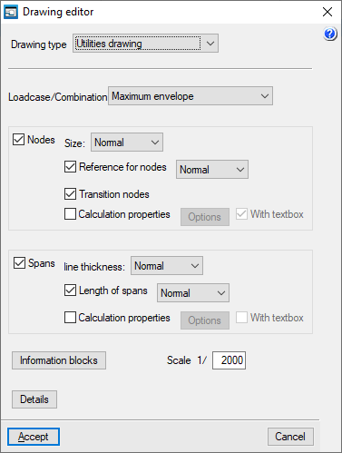
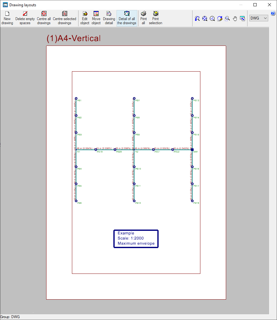
Utilities drawing
Shows the drawing of the installation on the plan.
The editing of the drawing offers the following options:
- Loadcase/Combination
Selects the loadcase, combination, envelope or oscillation for which data is to be displayed in the drawing. - Nodes (optional)
Displays the input information and analysis results of the nodes:- Size
- Node references (optional)
- Transition nodes (optional)
- Calculation properties (optional)
- Options: Flow, Depth, Ground level elevation, Elevation fill
- Spans (optional)
Displays the input information and analysis results of the spans:- Line thickness
- Length of spans (optional)
- Calculation properties (optional)
- Options: Dimension, Material, Flow, Pressure drop, Velocity
- Information texts
- General information table (optional)
- Quantities information table (optional)
- Excavation information table (optional)
- Scale
- Details
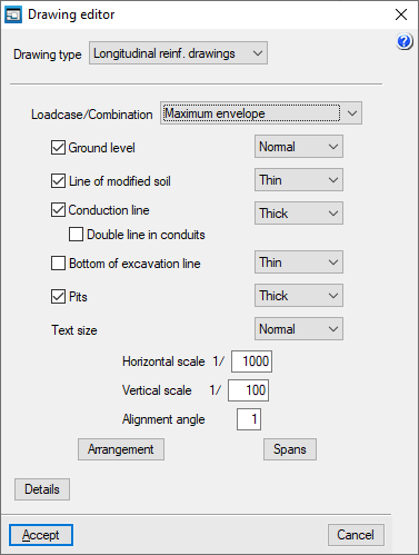
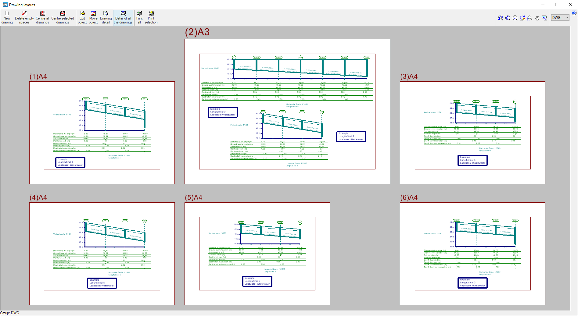
Longitudinal section drawings
Shows the longitudinal sections of the installation.
The editing of the longitudinal profile drawing offers the following options:
- Loadcase/Combination
Selects the loadcase, combination, envelope or oscillation for which data is to be displayed in the drawing. - Line thickness setting:
- Ground level (optional)
- Line of modified soil (optional)
- Conduction line (optional)
- Double line in conduits (optional)
- Línea de fondo de excavación (optional)
- Pits (optional)
- Text size
- Horizontal scale
- Vertical scale
- Alignment angle
- Arrangement
Edits the data to be displayed in the information arrangement under each longitudinal section. - Spans
Edits the data to be displayed on each section of the longitudinal section. - Details
GLTF file format compatible with BIMserver.center
If the job has been linked to a BIMserver.center project, a 3D model is generated in GLTF format to integrate the system model into the project when it is exported to the platform, allowing it to be visualised:
- on the online platform;
- on the BIMserver.center app for iOS and Android;
- on virtual reality and augmented reality;
- on other CYPE programs.
Integration into the BIMserver.center platform
Many of CYPE's programs are connected to the BIMserver.center platform and allow collaborative work to be carried out via the exchange of files in formats based on open standards.
Please note that, to work on BIMserver.center, users can register on the platform free of charge and create a profile.
When accessing a program connected to the platform, the program connects to a project in BIMserver.center. This way, the files of the projects that have been developed collaboratively in BIMserver.center are kept up to date.

| More information: |
|---|
| For further details related to using CYPE software via the BIMserver.center platform, please click on this link. |
Options available in CYPE Sewerage
At the top right of the auxiliary horizontal bar are the features required to use the program in conjunction with other BIMserver.center tools:

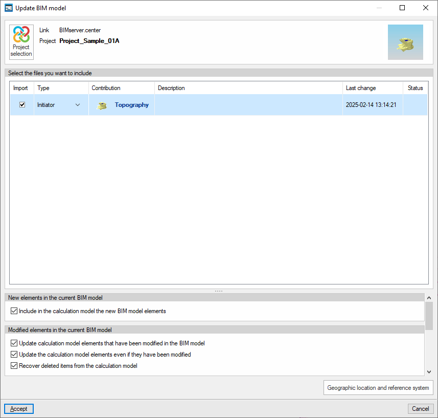
Update
Update the information contained in the files previously imported into the project, or import new files if required.
To do this, at the top, you must "Select the files you wish to include".
At the bottom, you can manage the inclusion of new elements or the updating and/or restoration of modified elements in the current BIM model by ticking the relevant boxes in the list.
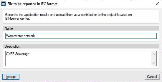
Export in "IFC" format
Export the information about the installation created using the program to BIMserver.center so that you can share it with other users.
During the export process, you can specify the details relating to the IFC file to be exported:
- Name
- Description
3D view
Clicking on this option displays a combined view of the models imported from the BIMserver.center project, alongside the elements specific to the installation drawn in the program.