Options in the "Properties" tab
The top tab "Properties" (accessible in the bottom tab "Structure") contains the options for defining the properties of nodes, bars and shells of the structure, as well as those for defining rigid diaphragms. It includes the following:
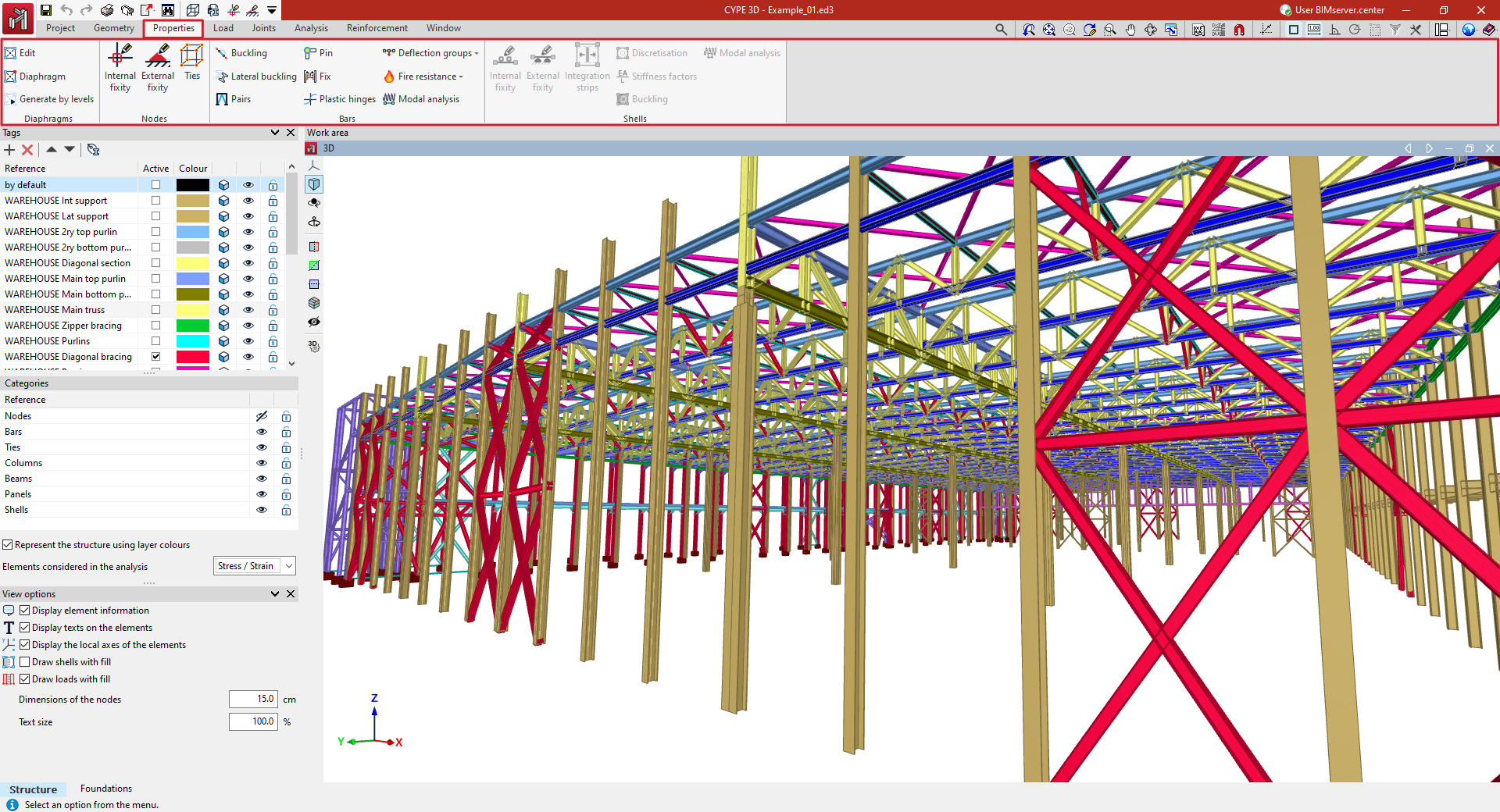
- in the "Diaphragms" group, the options for entering, generating and editing rigid diaphragms in the model;
- in the "Nodes" group, the options for editing the properties of the structure's nodes, such as defining internal and external connections or ties between nodes;
- in the "Bars" group, the options for editing bar properties, such as those related to buckling and lateral buckling, or entering bracing pairs, end connections and bracing, plastic hinges and deflection groups;
- and in the "Shells" group, the options for editing shell properties, such as the definition of internal and external ties or force integration strips.
Creating and editing rigid diaphragms
Rigid diaphragms are created and edited using the options available in the "Diaphragms" group on the top toolbar, within the "Properties" tab (under the "Structure" section).

Relative displacements between nodes belonging to the same rigid diaphragm are restricted. Therefore, each diaphragm can only rotate and move as a single unit.
This simplifies the analysis in structures where rigid diaphragms are assumed to exist, such as in each floor slab, which can be considered non-deformable in their plane.
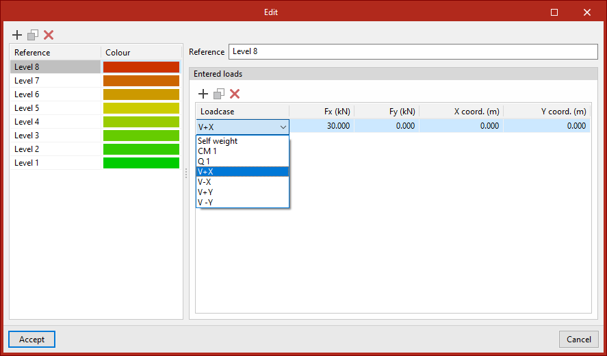
Edit
Allows you to manually create and/or edit the diaphragms, including their "Reference" and "Colour".
In addition, loads can be defined for each diaphragm. To do this, in the "Entered loads" table, you can select the "Loadcase", the load in the global X-direction ("Fx"), the load in the global Y-direction ("Fy") and the coordinates of the point of application ("X-coord." and "Y-coord.").
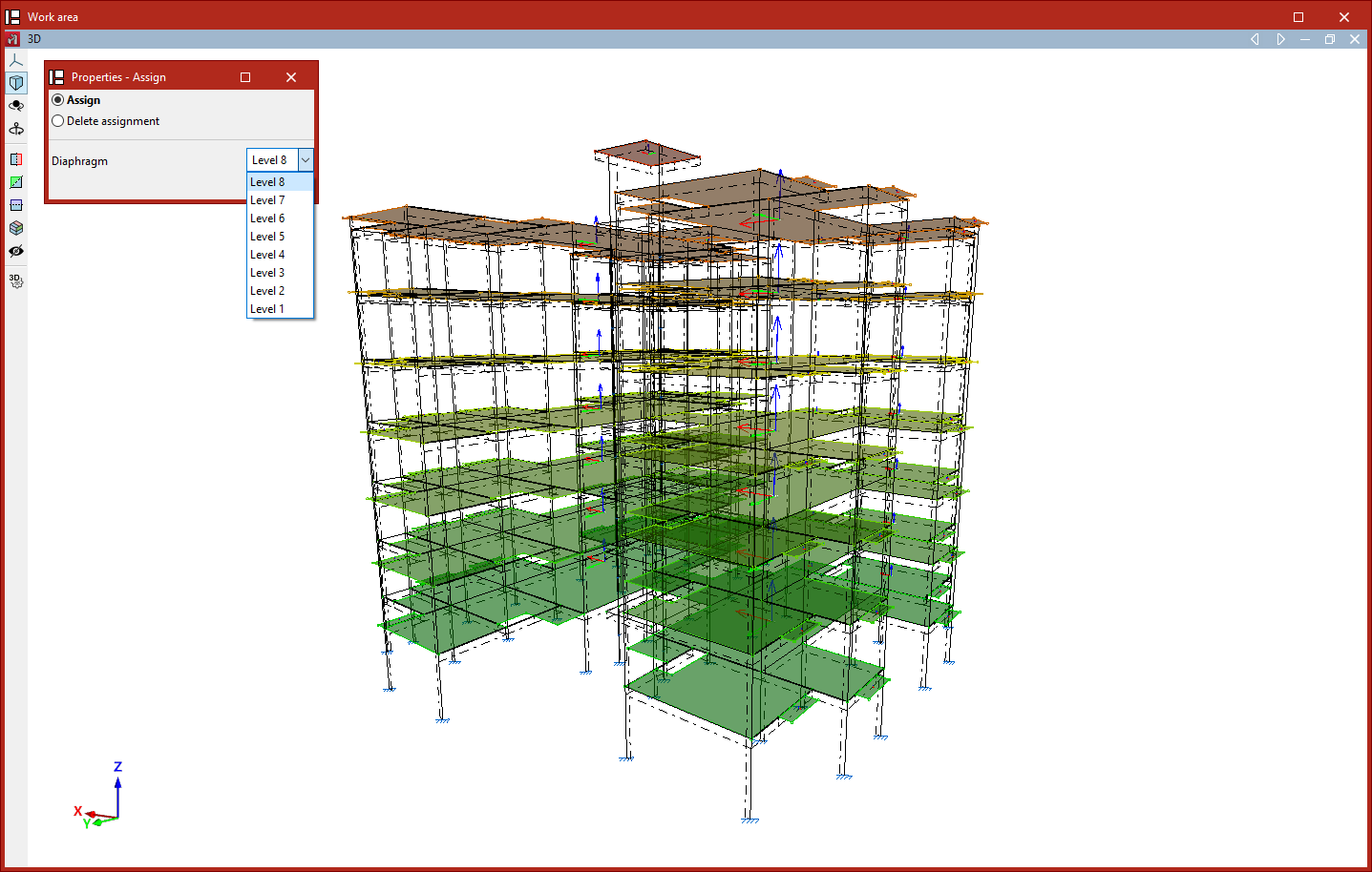
Diaphragm
This option allows you to "Assign" the "Diaphragm" selected from the drop-down menu to the nodes or shells selected in the workspace.
You can also "Remove assignment" by ticking the relevant option in the "Properties - Assign" pop-up window that appears when you select this option.
Generate by level
If levels have been defined in the project (using the "Levels" option in the "Planes" menu on the "Geometry" tab), this tool automatically generates a diaphragm for each level and assigns that diaphragm to all nodes on that level.
In the process, any previously defined diaphragms will be deleted. The program will display a dialogue box to warn you of this before continuing.
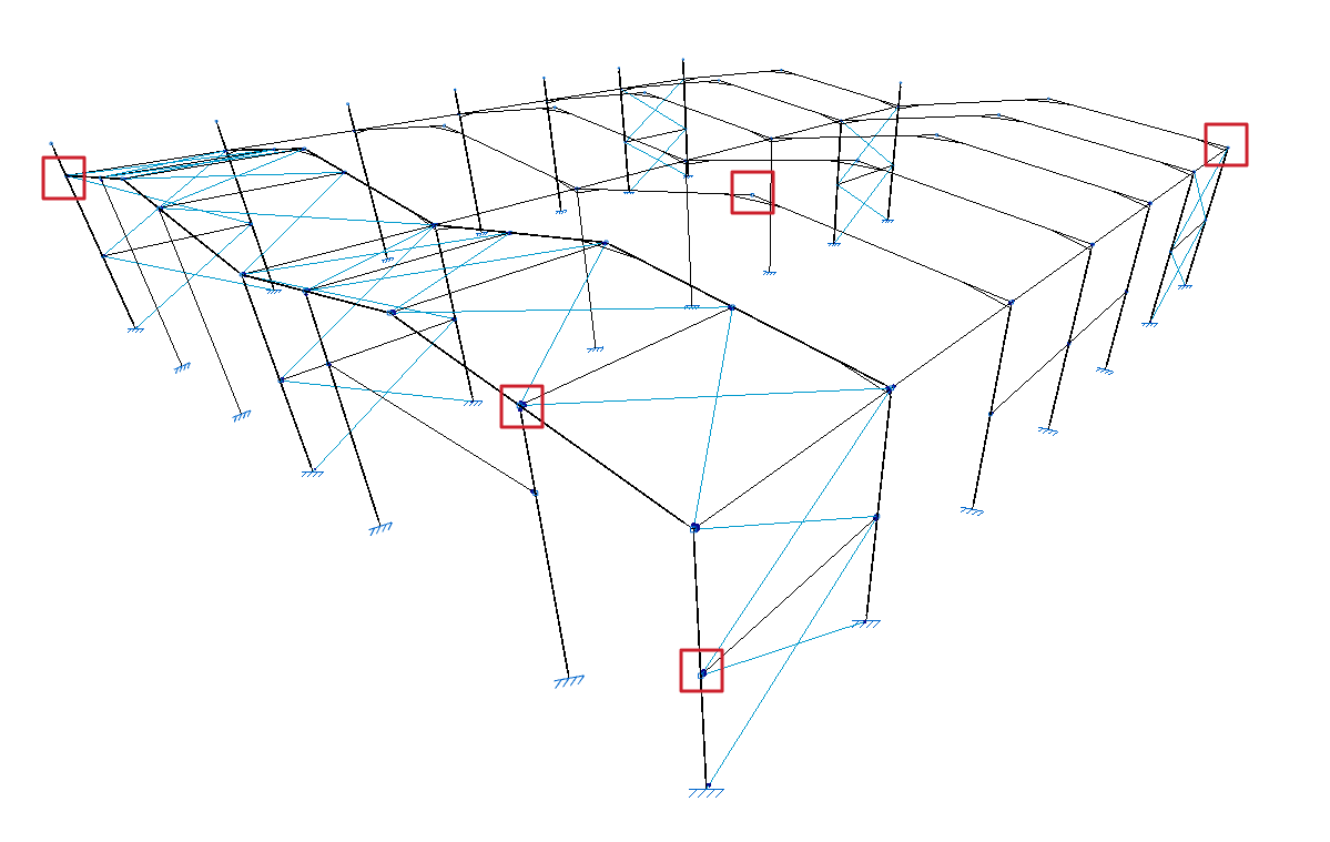
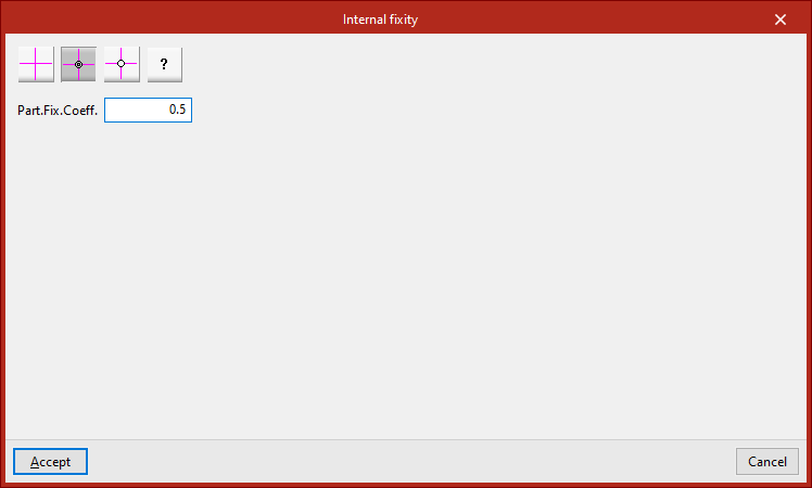
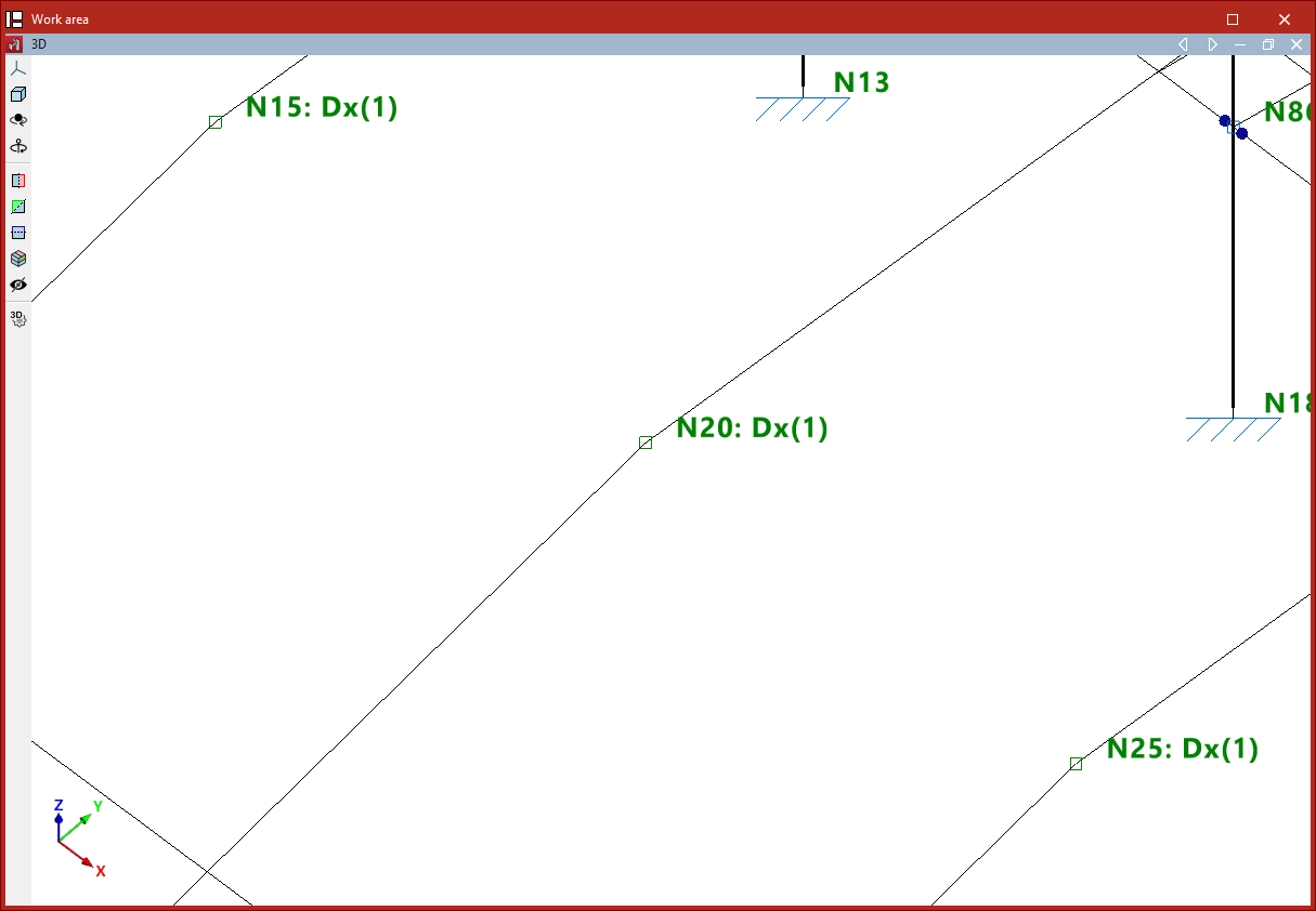
Defining internal fixity in nodes
The internal fixity in the nodes of the structure is defined with the following option, available in the "Nodes" group of the top toolbar, in the "Properties" tab (in the "Structure" tab).

Internal fixity
Enters internal fixity. Internal fixities are those that relate the ends of the bars that are connected to the same node.
To do this, after clicking on the option, select the nodes where the fixity is to be defined one by one or draw a selection box that covers them with the left mouse button. Finally, click on the right mouse button.
The program then opens a window where users can choose the type of internal fixity from the following:
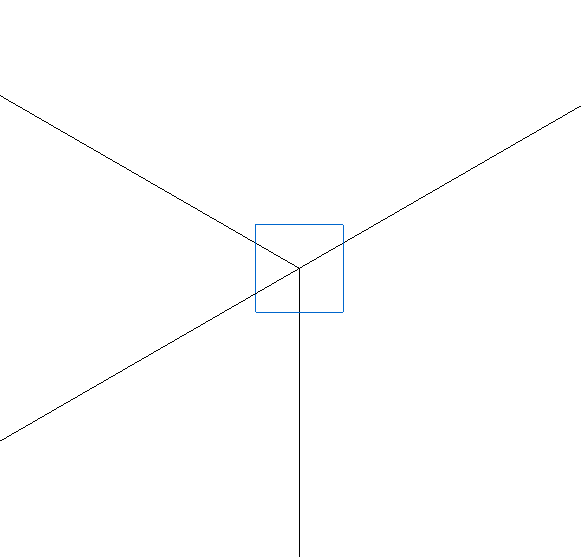
Fixed node
The "Fixed node" option defines a perfect fixity between all the bars that are connected to the node. As a result, they share the displacements and rotation angles in the design. This is the default option when entering new nodes or bars.
This is represented by a blue box symbol on the model display.
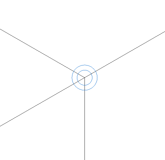
Fixed node with partial fixity coefficient for all its elements
The "Fixed node with partial fixity coefficient for all its elements" option is used to enter the partial fixity coefficient ("Part.Fix.Coeff.") which defines the degree of recessing between the parts that reach the node. The value can be between 0, which corresponds to a pinned connection, and a very large value, which corresponds to a fixity.
This is represented by the symbol of a double blue circle in the model display.
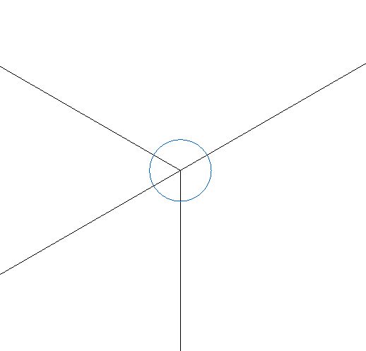
Pinned node
The "Pinned node" option defines a perfect link between all the elements that reach the node. In this case, the program uses a single blue circle above the node to represent the fixity.
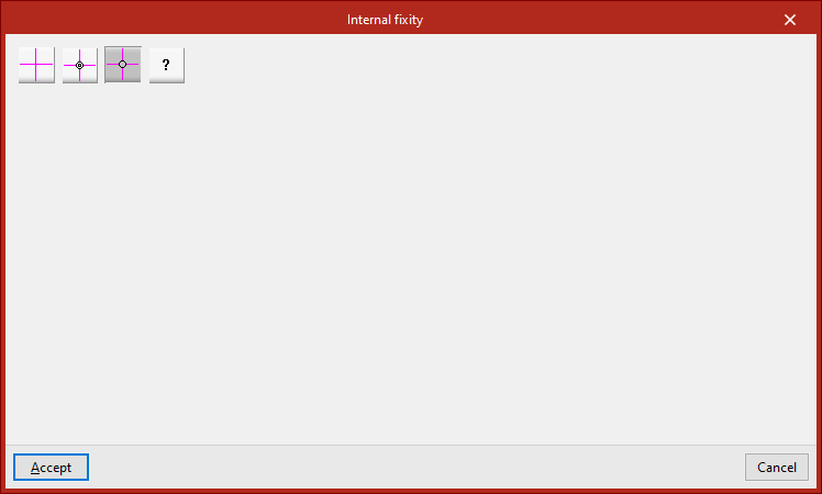
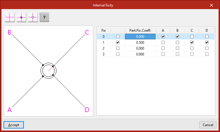
Generic node
The "Generic node" option is used to specify the degree of fixity between different groups of bars or shells that are attached to the node.
A diagram of the bars or shells is shown on the left. Each one is identified with the same reference letter as shown in the model display.
The table on the right describes the internal links between these elements. Each of the columns represents a bar or shell reaching the node and may have only one mark, which will be placed on one of the lines.
The bars or shells with the marking on the same line are embedded into each other and are linked with the rest of the bars or shells. In the diagram on the left, the elements embedded in each other are shown connected with the same circle.
If the box in the second column is activated, the elements with the same marking will be partially connected to the node. In this case, the value of the partial fixity coefficient ("Part.Fix.Coeff.") is written in the third column. This coefficient can take any positive value, with 0 corresponding to a joint.
If the box in the second column is unchecked, the program will not apply the defined partial embedding coefficient value.
In the diagram on the left, elements that are partially embedded are represented by a red line connecting them to the centre of the node.
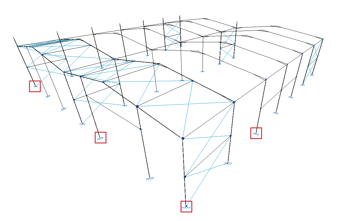
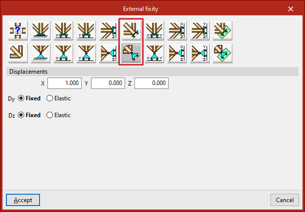
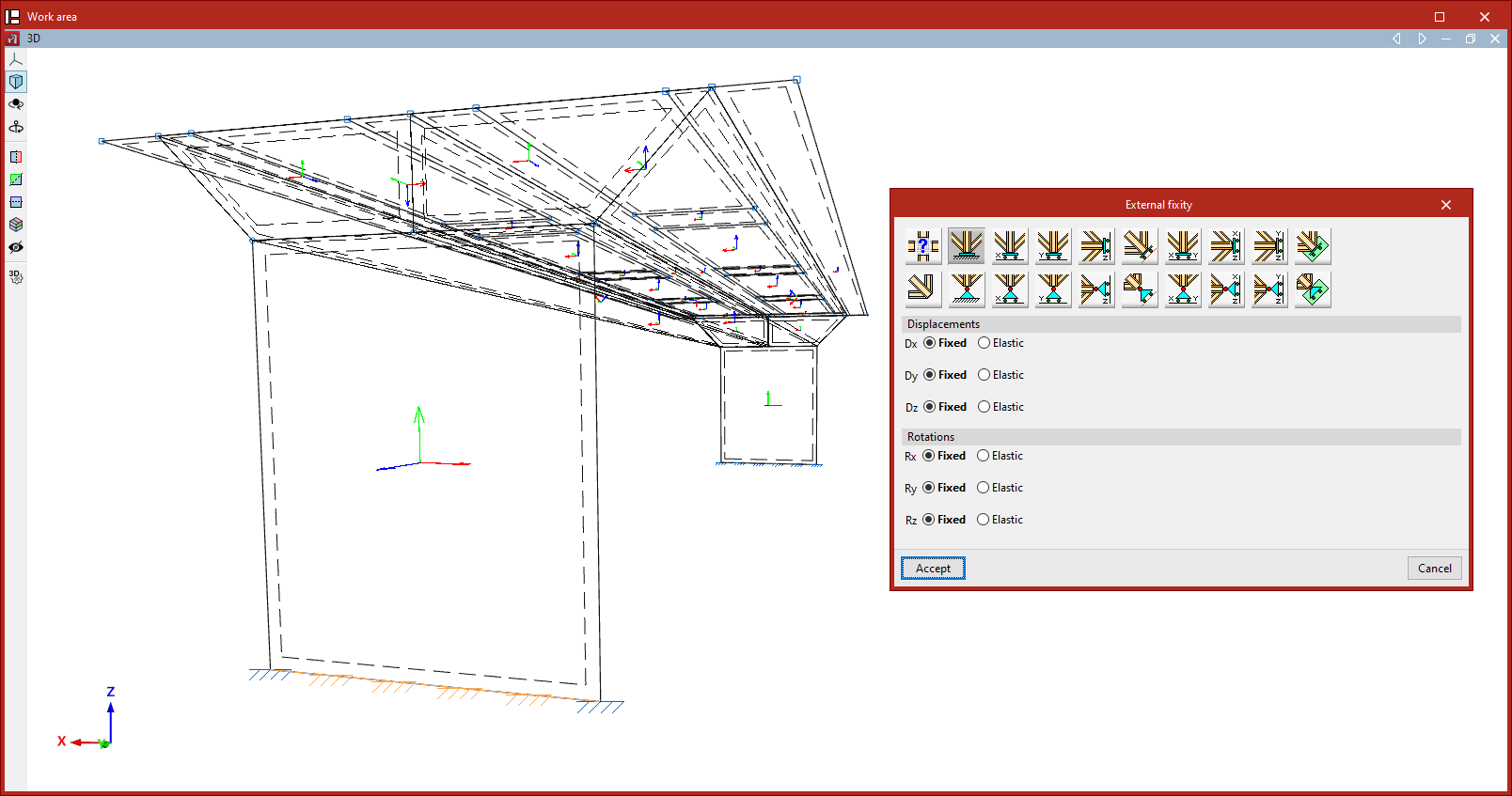
Defining external fixity in nodes
The external fixity in the nodes of the structure is defined with the following option, available in the "Nodes" group of the top toolbar, in the "Properties" tab (in the "Structure" tab).

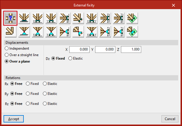
External fixity
Enters external fixity. External fixities restrict the displacement or rotation of the nodes of the structure and correspond to the supports on the ground and on other elements outside the model.
To do this, after clicking on the option, select the nodes where the connection is to be defined one by one or draw a selection box that covers them with the left mouse button. Finally, click on the right mouse button.
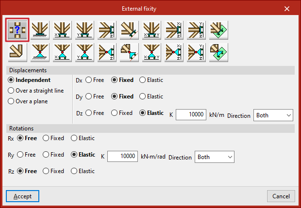
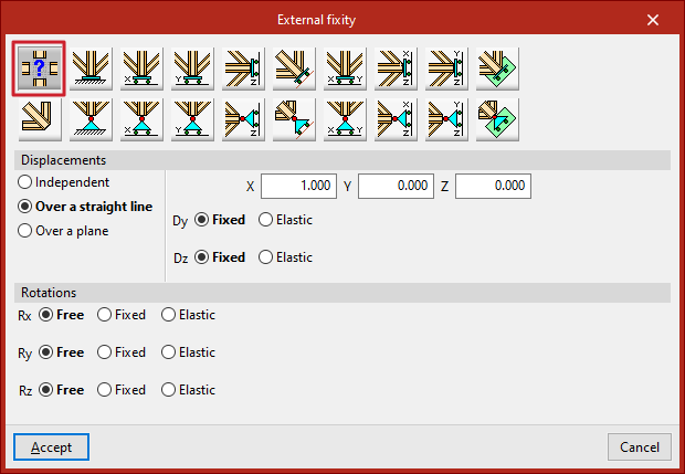
The program will open a window where the type of "External fixity".
Free
By default, a newly inserted node will be "Free", i.e. it will not have any external fixities.
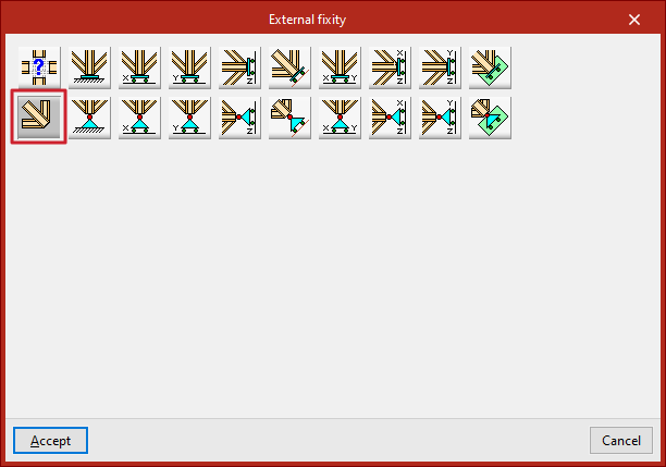
The other options are used to define external fixity in the node.
Generic
The "Generic" option manually defines the restrictions on "Displacements" and "Rotations" in the three directions of the space.
Displacements
"Displacements" can be "Independent", "Over a straight line" or "Over a plane".
In case they are defined as "Independent", the behaviour of the displacements in the three axes, "Dx", "Dy" and "Dz", is specified:
- If "Free", the displacement in that direction shall not be constrained.
- If "Fixed", the displacement is constrained and takes a fixed value. By default, this value is null, unless the "Prescribed displacements" option has been used from the "Load" tab, in which case it will assume this value.
- If "Elastic" is selected, the program assumes an elastic support in that direction. On the right, the elastic constant of the support is written in the units indicated, and its "Direction" is specified (it can act in "Both" directions or only in "Negative" or "Positive" directions).
If the "Displacements" are defined "Over a straight line", the node can only be displaced in the direction of the director vector defined by the X, Y and Z components entered on the right. In the directions perpendicular to this line, users specify whether the support is "Fixed" or "Elastic".
If the "Displacements" are defined "Over a plane", the node can only be displaced in the plane perpendicular to the vector defined by the X, Y and Z components entered. Similarly, in the direction perpendicular to the plane, users indicate whether the support is "Fixed" or "Elastic".
Rotations
In the "Rotations", "Gx", "Gy" and "Gz", choose "Free" if the rotation is not constrained in the indicated direction, "Fixed" if the rotation is constrained and takes a fixed and null value, or "Elastic" if the constraint to the rotation is elastic, in which case the constant governing the rotational stiffness of the support must be written and, in addition, its "Direction" is specified (it may act in "Both" directions or only in "Negative" or "Positive" directions).
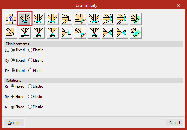
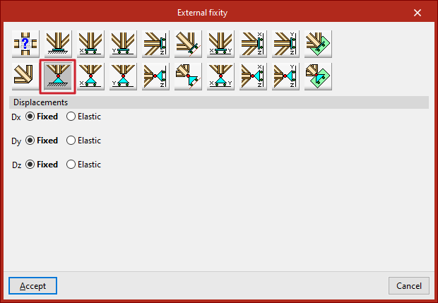
The other options in the "External fixity" panel correspond to predefined external fixities that simplify data entry to speed up the process.
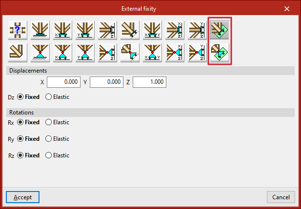
Fixity
The "Fixity" option prevents "Displacements" ("Dx", "Dy" and "Dz") and "Rotations" ("Gx", "Gy" and "Gz") in the three directions of the selected node.
Each prevented displacement or rotation must be defined as "Fixed" or "Elastic".
Pinned connection
The "Pinned connection" option prevents only the "Displacements" ("Dx", "Dy" and "Dz") in the three directions of the selected node.
Each prevented displacement or rotation must be defined as "Fixed" or "Elastic".
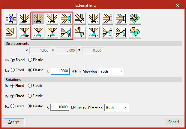
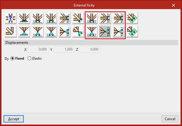
Free displacements on a straight line in X, Y or Z directions
These options define free displacements over a straight line in the global directions X, Y or Z.
The options in the first row constitute freely movable fixities and also constrain the rotation:
- Free displacement over a straight line in X direction
- Free displacement over a straight line in Y direction
- Free displacement over a straight line in Z direction
Those in the second row constitute supports with free displacement and hold the rotations without constraint:
- Free displacement over a straight line in the X direction with unrestrained rotations
- Free displacement over a straight line in the Y direction with unrestrained rotations
- Free displacement over a straight line in the Z direction with unrestrained rotations
In all these cases, the components of the line's director vector are already defined in the numerical fields in grey. Users simply indicate whether the displacement or rotation in each of the directions shown is "Fixed" or "Elastic".
Free displacements over any straight line
The following options define a free displacement over any straight line, with coerced rotations or with uncoerced rotations:
In all these cases, the components of the line's director vector are already defined in the numerical fields in grey. Users simply indicate whether the displacement or rotation in each of the directions shown is "Fixed" or "Elastic".
Free displacements on a plane parallel to the XY, XZ or YZ axes
The following options are used to define free displacements in a plane parallel to the global XY, XZ or YZ axes.
The options in the first row constitute freely displacement fixities and also constrain rotations:
- Free displacement in a plane parallel to XY axes
- Free displacement in a plane parallel to XZ axes
- Free displacement in a plane parallel to YZ axes
Those in the second row constitute supports with free displacement and hold the rotations without constraint:
- Free displacement in a plane parallel to the XY-axes with unconstrained rotation
- Free displacement in a plane parallel to the XZ-axes with unconstrained rotation
- Free displacement in a plane parallel to the YZ-axes with unconstrained rotation
In all these cases, the components of the vector perpendicular to the plane are already defined in the numerical fields in grey. Users simply indicate whether the displacement or rotation in each of the directions shown is "Fixed" or "Elastic".
Free displacements over any plane
Finally, a free displacement on any plane can be defined, with forced or uncoerced rotations:
- Free displacement in any plane
- Free displacement in any plane with unconstrained rotations
The components of the vector perpendicular to the plane must be entered and users must indicate whether the displacement or rotation in each of the directions shown is "Fixed" or "Elastic".
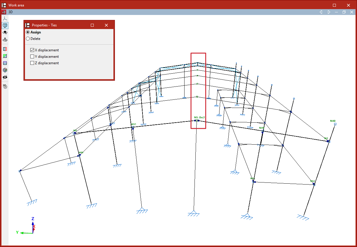
Defining node ties
The assignment and removal of node ties is carried out using the following option, available in the "Bars" group on the top toolbar, under the "Properties" tab (in the "Structure" tab).

Node ties are used to enforce that two or more nodes have identical displacements in all load cases.
To apply this condition, the actual structure must include some element or construction detail that effectively guarantees the equality of displacements, even if it is not graphically represented in the model.
Assigning ties
After clicking on "Ties", in the "Properties – Ties" window, if "Assign" is selected, you can choose whether to equalise "X displacement", "Y displacement", or "Z displacement". These directions refer to the global axes.
Displacements can be equalised in one, two, or all three directions simultaneously by checking the corresponding boxes.
After selecting the desired options, proceed to select the nodes to be tied by clicking on them one by one with the left mouse button or by defining a selection area.
Then, right-click to confirm the selection.
Once this is done, a text will appear next to the node reference indicating the existence of a tie in each spatial direction, along with an ID number used to differentiate the various groups of nodes with tied displacements.
This information can also be viewed by hovering the pointer over the corresponding node.
Deleting ties
You can "Assign" new ties and "Delete" existing ones from the "Properties – Ties" window.
First, select the directions in which you want to remove the ties.
Then, select the nodes one by one using the left mouse button or by defining a selection area.
Upon right-clicking, the node will lose the ties previously defined in the selected directions.
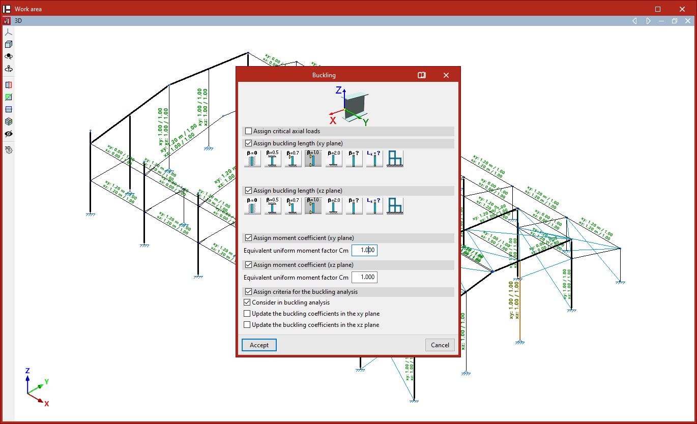
Editing the buckling parameters of the bars
The buckling parameters for the bars are defined using the following option, which is available in the "Bars" group on the top toolbar, within the "Properties" tab (under the "Structure" section).

Buckling
The "Buckling" option allows you to edit the parameters relating to the buckling of the bars.
After clicking on the option, select each bar by clicking on them one by one, or highlight a capture area. Then, right-click.
In the window that appears, you can define the buckling parameters in two different ways:
- If the "Assign critical axial loads" checkbox remains unchecked, the buckling lengths (or buckling coefficients) of the bar are entered, along with the moment coefficients in the local XY and XZ planes. In this case, the critical axes of the bar are calculated automatically by the program.
- If the "Assign critical axial loads" checkbox is checked, you can enter the values for the critical buckling axes, as well as the moment coefficients in the local XY and XZ planes.
To make it easier to identify the buckling planes, the diagram above shows the local coordinate axes of the section, using the same colour coding as in the model.
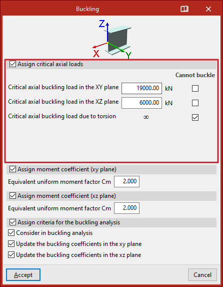
Assigning critical axial loads
To assign critical axial loads, tick the "Assign critical axial loads" box.
This section allows you to manually enter the values for the critical axial buckling loads as an alternative to the buckling lengths:
- Critical axial buckling load in the XY plane
- Critical axial buckling load in the XZ plane
- Critical axial buckling load due to torsion
The "Cannot buckle" checkbox can be ticked in any section. In this case, an infinite critical axis is assumed.
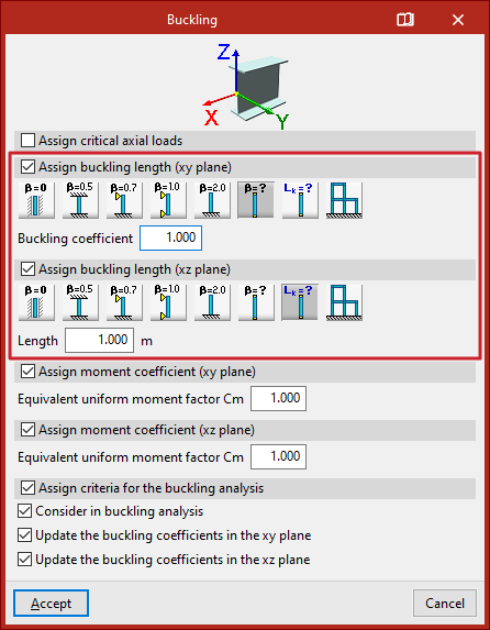
Assigning buckling lengths or buckling coefficients
If you choose to assign buckling lengths or buckling coefficients, the "Assign critical axial loads" checkbox is deselected.
The program then allows you to assign buckling lengths or buckling coefficients to each local plane of the section by ticking the relevant boxes (“Assign buckling length (xy plane)” and “Assign buckling length (xy plane)”).
If you choose to define the buckling coefficient (beta), this value will be multiplied by the length of the bar from node to node to obtain the buckling length.
The available options include the following:
- Do not take buckling into account
In this case, the program uses a default value of 0 for the buckling coefficient. - Beam fixed at both ends
A buckling coefficient of 0.5 is assumed. - Bar, simply supported at one end and fixed at the other
A buckling coefficient of 0.7 is used. - Simply supported bar
A buckling coefficient of 1 is assumed. This is the default selection made by the program. - Cantilever bar
A buckling coefficient of 2 is assumed. - Other buckling coefficient values
This option allows you to manually enter the "Buckling coefficient" in the field below, rather than using one of the predefined values. - Assign buckling length
This option allows you to enter the buckling length directly, rather than using a coefficient to multiply the bar length. To do this, select the relevant option and enter the "Length" value in the units of measurement defined in the project. The buckling length corresponds to the distance between two consecutive inflection points in the bar’s deformed shape. - Approximate calculation of buckling lengths
This option allows you to perform an approximate calculation of buckling lengths, specifying whether the structure is a "Sway frame" or "Non-sway frame" type. The validity of this approximate analysis is limited to substantially orthogonal structures. There are other conditions and limitations for this analysis, which can be found in the help text that appears when you hover the pointer over the option.
| Note: |
|---|
| The approximate analysis of buckling lengths is based on commonly accepted formulas whose validity is limited to substantially orthogonal structures. The user must specify, at their discretion, whether the structure is translational or intranslational. Furthermore, the following assumptions are accepted - The supports buckle simultaneously - Elastic shortening of the supports is neglected - The beams behave elastically and are rigidly connected to the supports - The stiffness of the beams is not altered by normal forces. There are a number of limitations regarding the validity of the buckling coefficient results provided by this method, which must be taken into account - The presence of intermediate nodes in continuous bars, to which no other bars are connected, invalidates the method; therefore, in such cases, the necessary manual corrections must be made. - The method requires the structure to be classified as translational or intranslational; care must therefore be taken with this definition. - If the structure entered is a plane frame, the values obtained are valid in its plane but may not be valid in the perpendicular plane (for example, because bracing elements exist in reality that are not defined in the calculated structure). |
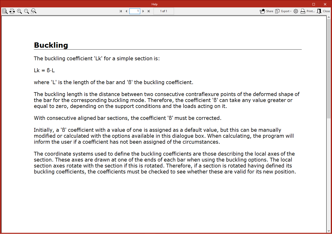
Assignment of moment coefficients
You can then enter the moment coefficients in the local XY and XZ planes.
To do this, tick the boxes "Assign moment coefficient (xy plane)" and/or "Assign moment coefficient (xz plane)", then enter the "Equivalent uniform moment factor Cm" for each plane.
Each standard provides values for these coefficients based on the different bending moment distributions between bracing points.
By default, the program uses coefficients equal to one.
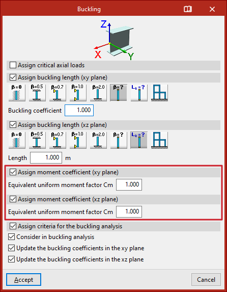
Assignment of criteria for buckling analysis
The "Assign criteria for the buckling analysis" section relates to the linear buckling analysis performed by the program using the options in the "Buckling" group on the "Analysis" tab. This analysis allows the buckling coefficients of the bars to be obtained and updated automatically.
This section contains three options:
- Include in buckling analysis
By ticking or unticking this box, you can specify whether or not the bar is included in the buckling analysis. - Enable updating of buckling coefficients in the XY
plane
Ticking this box allows the program to update the bars' buckling coefficient in the local XY buckling plane. - Enable updating of buckling coefficients in the XZ
plane
Ticking this box allows the program to update the bar’s buckling coefficient in the local XZ buckling plane.
Updating the buckling coefficients requires a buckling analysis to be carried out. When assigning buckling coefficients to the bars, the program will automatically select "Other buckling coefficient values" and enter the updated buckling coefficient values in the "Buckling coefficient" field in this window.
| Note: |
|---|
| You can manually set the buckling coefficient and disable the option to update the coefficients so that the program does not modify them; for example, if you wish to force the program to assume that a bar does not buckle in a particular plane because it is braced. If these boxes are left ticked, the program will assign the buckling coefficients based on the calculation performed. |
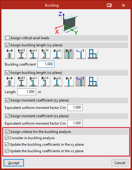
Results
Finally, click "Accept". As you move closer to the bars, the program displays text above them showing the parameter values entered for the XY plane and the XZ plane.
This information is also displayed in the pop-up window that appears when you hover the cursor over the bars, under the "Buckling" section. Furthermore, it indicates whether the bar is "Included in the buckling analysis" or not.
If no coefficients have been assigned to the bars when clicking "Analyse", the program displays a "Warning" message to this effect. If you continue, the default values will be used.
| Note: |
|---|
| Buckling parameters have a significant impact on certain bar checks. These checks vary depending on the selected code and can be viewed in the "U.L.S Checks" lists under the "Analysis" tab. Examples include the "Compression resistance" and "Combined bending and axial resistance" checks. |
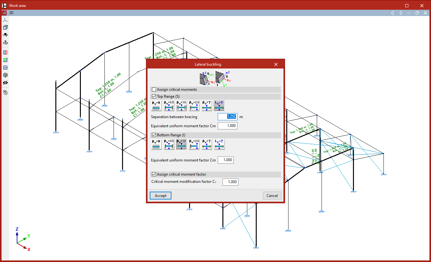
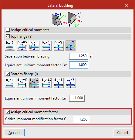
Editing the lateral buckling parameters of the bars
The lateral buckling parameters for the bars are defined using the following option, which is available in the "Bars" group on the top toolbar, within the "Properties" tab (under the "Structure" section).

Lateral buckling
The "Lateral buckling" option allows you to edit the parameters relating to the lateral buckling of the bars.
After clicking on the option, select each bar by clicking on them one by one, or highlight a capture area. Then, right-click.
In the window that appears, you can define the lateral buckling parameters in two different ways:
- If the "Assign critical moments" checkbox remains unchecked, the lateral buckling lengths (or lateral buckling coefficients) of the bar must be entered, along with the modification factor for the critical moment. In this case, the critical moments of the bar are calculated automatically by the program.
- If the "Assign critical moments" checkbox is checked, you can enter the values for the critical lateral buckling moments, and the modification factor for the critical moment.
The diagram above shows the positions of the upper and lower flanges of the section in relation to the orientation of the local coordinate axes, using the same colour coding as in the model.
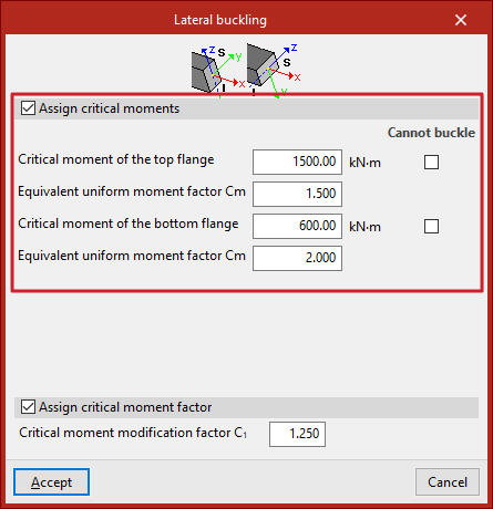
Assignment of critical moments
If you choose to assign critical moments, tick the "Assign critical moments" box.
This section, available for rolled and formed steel bars, allows you to manually enter the values of the critical lateral buckling moments as an alternative to the lateral buckling lengths:
- Critical moment for the top flange
- Equivalent uniform moment factor Cm (for the top flange)
- A critical moment of the bottom flange
- Equivalent uniform moment factor Cm (for the bottom flange)
The "Cannot buckle" checkbox can be selected for any flange. In this case, an infinite critical moment is assumed.
The "Assign critical moment factor" option is available for the following standards:
- Eurocodes 3 and 4
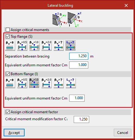
Assignment of lateral buckling lengths or lateral buckling coefficients
If you choose to assign lateral buckling lengths or lateral buckling coefficients, the "Assign critical moments" checkbox is deselected.
You can then define the lateral buckling parameters for the "upper flange" and "lower flange" of the section by ticking the relevant boxes.
If you choose to define the lateral buckling coefficient, this value will be multiplied by the length of the bar from joint to joint to obtain the lateral buckling length, or the spacing between bracing bars.
The options available in each flange include the following:
- Does not check for lateral
buckling. In this case, the program uses a predefined value for the lateral buckling coefficient, set to 0. This is the default value. Consequently, the program does not take lateral buckling into account. - Well-braced beam
A lateral buckling coefficient of 0.5 is assumed. - Self-supported beam
A lateral buckling coefficient of 1 is assumed. - Cantilever beam
A lateral buckling coefficient of 2 is assumed. - Lateral buckling coefficient
This allows you to enter the value of the lateral buckling coefficient manually instead of using one of the predefined values. To do this, enter the value in the field below. - Spacing between bracing bars
This allows you to enter the spacing between bracing bars or the lateral buckling length of each flange directly, rather than using a coefficient. To do this, select the relevant option and enter the value in the units of measurement defined in the project.
In addition, the program allows you to enter the "Equivalent moment coefficient" for each of the flanges.
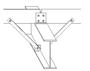
The installation of flange fasteners, such as these struts, allows for a lower lateral buckling coefficient or bracing spacing to be used. For example, if these elements are positioned at the midpoint of the section’s length, it may be justified to use a lateral buckling coefficient of 0.5.
Assignment of the modification factor for the critical moment
Finally, you can tick the "Assign critical moment factor" box to enter the "Modification factor for the critical moment".
Each standard provides values for the equivalent moment coefficients and for the critical moment adjustment factor based on the different bending moment distributions in the bars between bracing points.
By default, the program uses coefficients equal to one.
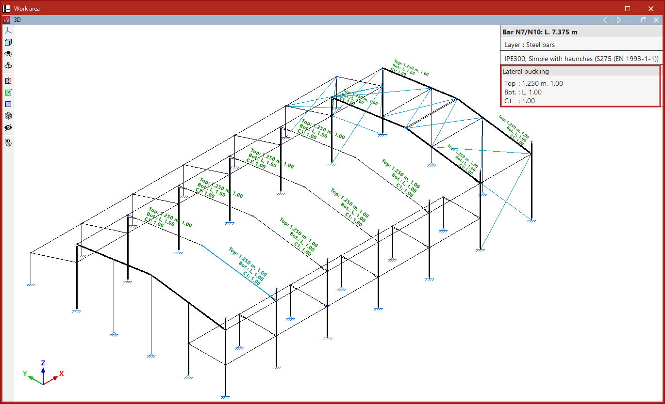
Results
Finally, click "Accept". When you hover over the bars, the program displays text above them showing the values of the parameters applied to the two flanges and the value of the critical moment factor.
This information is also displayed in the pop-up box that appears when you hover the cursor over the bars, under the "Lateral buckling" section.
If no lateral buckling parameters have been assigned to the bars when clicking "Analyse", the program displays a "Warning" message to this effect. If you continue, the default values will be used.
| Note: |
|---|
| Lateral buckling parameters have a significant impact on certain bar checks. These checks vary depending on the selected code and can be found in the "U.L.S checks" reports under the "Analysis" menu. Among these, the "Y-axis bending resistance" check is worth mentioning. |
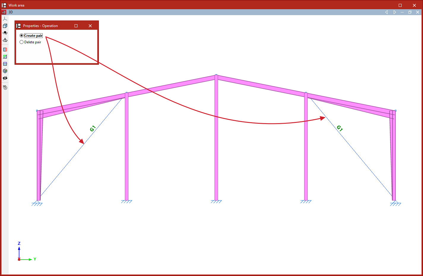
Defining bracing pairs for buckling analysis
Bracing pairs for buckling analysis are defined using the following option, which is available in the "Bars" section of the top toolbar, within the "Properties" tab (under the "Structure" tab).

Pairs
The "Pairs" option allows you to define pairs of bracing elements that are not located within the same braced frame, so that they can be taken into account in the buckling analysis.
To do this, after clicking on the option, select "Create pair" in the "Properties - Operation" window. Next, select the two elements in the model defined with "Only tension" behaviour (defined in the "Behaviour" drop-down menu in the "Describe" window, accessible when creating each element or when editing them via the "Section" option on the "Geometry" tab) that form the bracing pair.
The program will indicate the presence of each bracing pair with an identifying label on the beams.
You can also select "Delete pair" in the "Properties - Operation" window to remove the definition of a bracing pair. In this case, simply click on either element of the pair to delete it.
In the analysis, if both elements of a bracing pair are subjected to compression under the same load case, they will be treated as such in the buckling analysis, with their axial stiffness reduced by half, in a similar way to how the software automatically handles elements with "tension-only" behaviour that are located within the same braced frame.
| Note: |
|---|
| Linear buckling analysis is performed for each loadcase by removing non-linear elements that do not contribute to the analysis and converting those that do into equivalent linear elements. In this process, when two elements with "tension-only" behaviour form a braced frame, and both elements are in compression under the same loadcase, the program transforms the behaviour of these elements to linear and reduces their axial stiffness by half. By default, in situations where a frame is braced by two non-intersecting elements, and both are in compression under the same load case, the program removes them before performing the buckling analysis; consequently, the results of this analysis are obtained without taking them into account. |
Fitting pins at the ends of the bars
The pins at the ends of the beams are created using the following option, available in the "Beams" section of the top toolbar, within the "Properties" tab (under the "Structure" sub-tab).

Pins
The "Pin" option allows you to add pins to the ends of the bars, enabling full rotation in all three spatial directions, including rotation about their own axis.
When you click on the option, a pop-up window will appear asking whether you wish to make a "Single" or "Multiple" selection.
If an "Individual" selection is made:
- When you click in the middle of a bar, the program inserts pins at both ends.
- If you click on one end of a bar, the pin is only inserted at that point.
- To remove the pins you have inserted, click again on the centre or end of the bars.
If a "Multiple" selection is made, the program will add or remove pins at both ends of the selected bars.
In the model, the articulated ends are represented by blue circles.

| Note: |
|---|
| The "Pin" option does not allow you to define any partial fixity. To do this, you must use the "Fix" option in the same group of options. |
Defining the fixing conditions at the ends of the bars
The fixing conditions at the ends of the bars are defined using the following option, available in the "Bars" section of the top toolbar, within the "Properties" tab (under the "Structure" tab).

Fixing
The "Fix" option allows you to define the conditions for full or partial fixed ends at the ends of the bars, in the local XY, XZ and YZ planes.
When this option is selected, the program displays text at the ends of the beams showing the support values defined for the XY, XZ and YZ planes.
This information is also shown in the table that appears when you hover over the components, under the "Fixity at ends" section.
To change the values, select the parts by clicking on them one by one or using a selection window. Then, right-click.
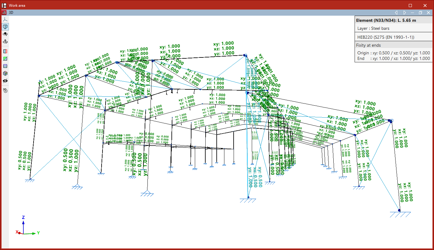
In the "Fixity at ends" pop-up window, tick the "Assign (xy plane)", "Assign (xz plane)" and/or "Assign (yz plane)" boxes to specify the local plane in which you wish to modify the embedding.
On the right, the program displays two columns where these conditions can be defined for the "Origin of the element" and the "End of the element".
In each case, you can choose to enter a "Fixity coefficient" or a "Rotational stiffness".
| Note: |
|---|
| The fixed-end coefficients can take values between 0 (if the end is fully pinned) and 1 (if it is fully fixed). Intermediate values correspond to partially fixed ends. By default, the program assigns a fixed-end coefficient of 1 at both ends. |
If you wish to define an elastic internal connection, select the "Rotational stiffness" option and enter the corresponding value.
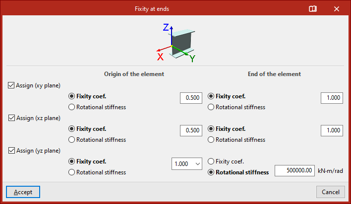
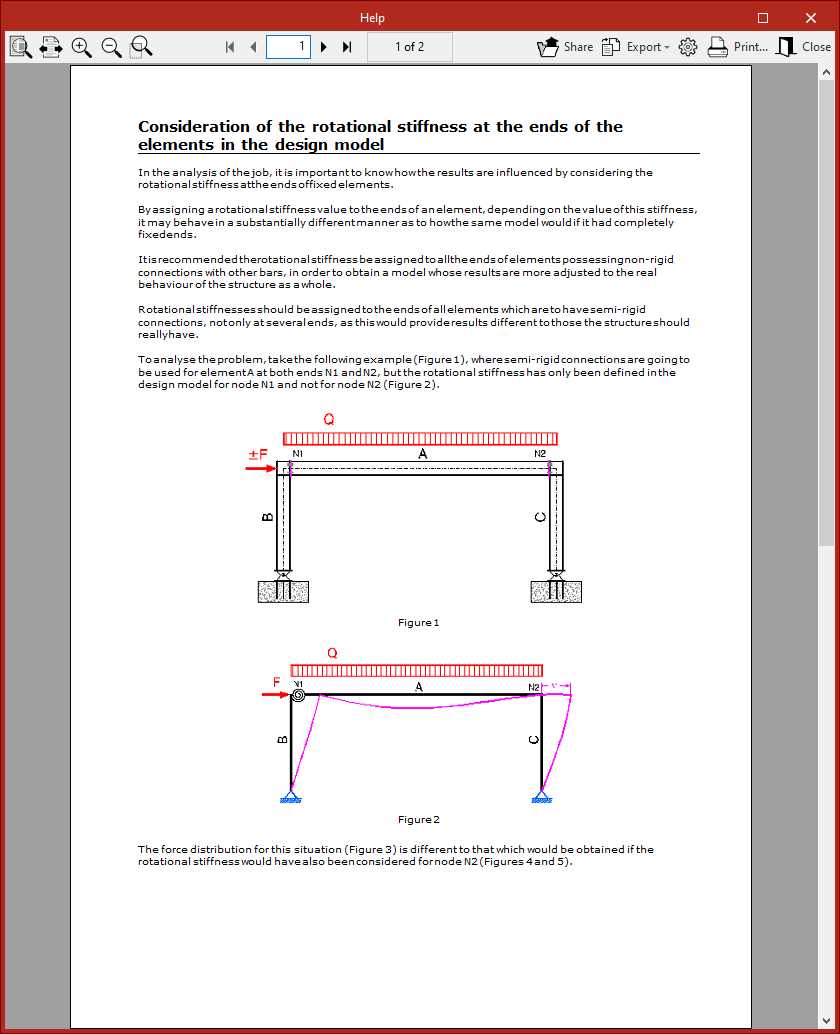
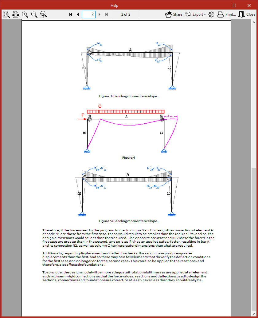
You can click the "Show detailed information relative to the use of this dialogue box" button in the title bar of the pop-up window to find out more about the "Consideration of the rotational stiffness at the ends of the elements in the design model".
Finally, click "Accept" to apply the changes.
Inserting and editing plastic hinges in bars
Plastic hinges can be inserted and edited in bars using the following option, which is available in the "Bars" section of the top toolbar, within the "Properties" tab (under the "Structure" sub-tab).

Plastic hinges
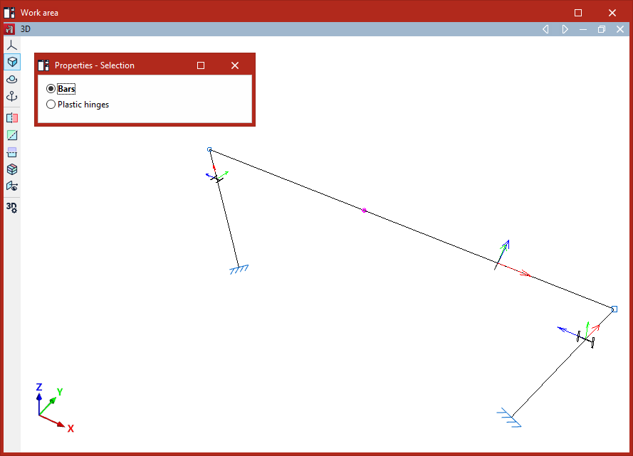
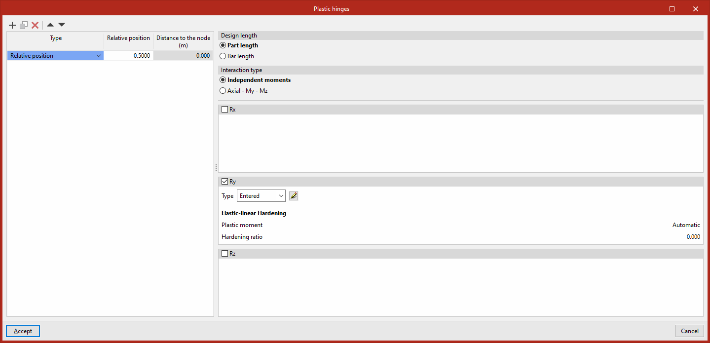
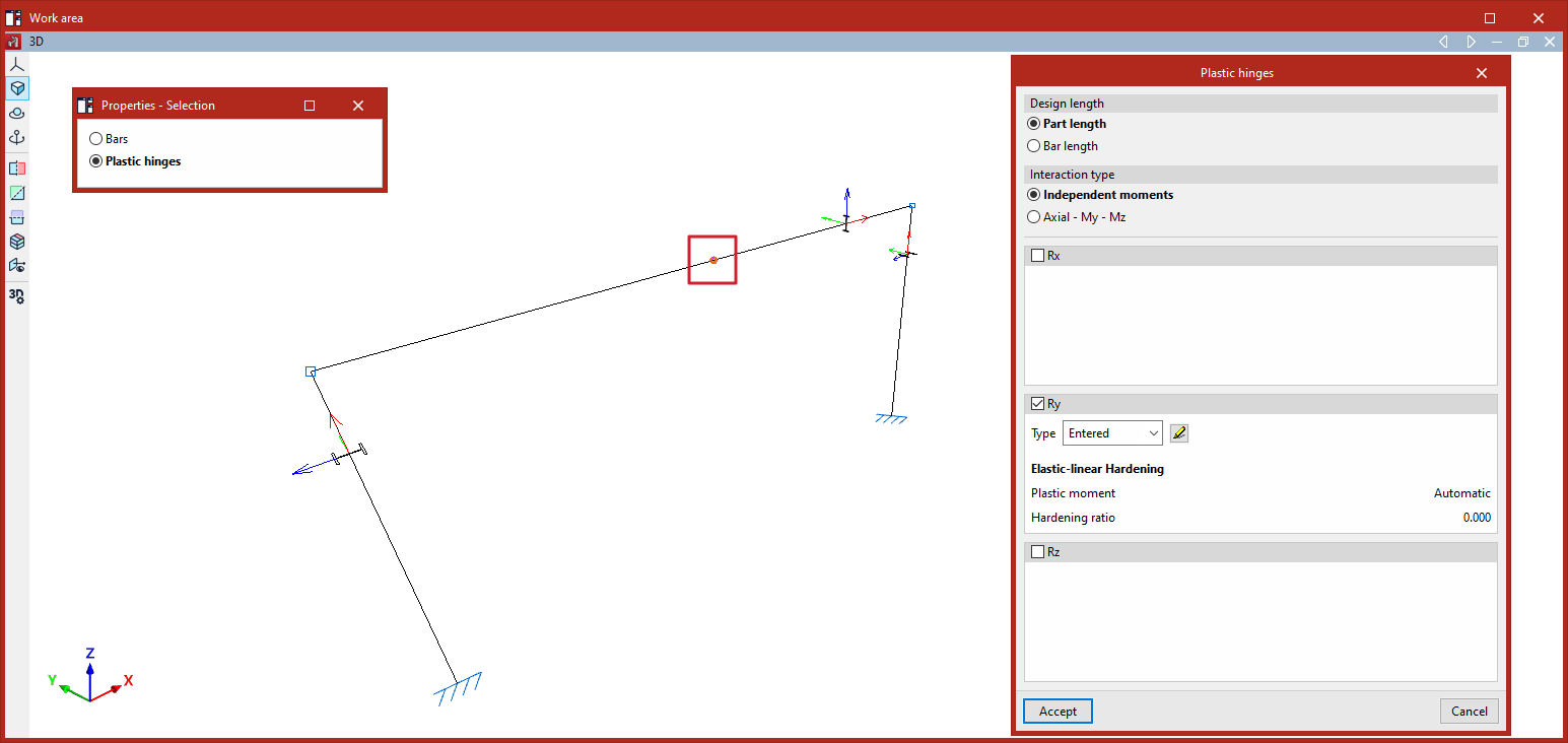
After clicking on the "Plastic hinges" option, the program opens the "Properties - Selection" window, which offers two options: "Bars" or "Plastic hinges".
Entering plastic hinges
If you select "Bars", you can insert plastic hinges into a group of bars.
To do this, select the bar or group of bars using the left mouse button, then click the right mouse button.
A list will then appear where you can "Add", "Copy", "Delete" or reorder plastic hinges on the bars using the buttons at the top.
The "Type" drop-down menu allows you to specify the source of the data:
- Relative position
In this case, the "Relative position" of each hinge in the bar is defined by entering a value between 0 and 1. - Regarding the initial node
- Regarding the final node
If either of these two options is selected, the “Distance to node” indicated for each joint must be entered in the bar.
The properties of each hinge selected from the list are specified on the right. Thus, under "Design length", you must specify whether to use the "Part length" or the "Bar length".
The "Interaction type" specifies whether the hinge considers "Independent moments" or the axial–moment–moment interaction ("Axial - My - Mz"). The first option assumes that the axial force remains constant and is a simplification that usually provides sufficiently accurate results in many cases:
- For independent moment hinges, the degrees of rotational freedom in which they act (expressed in the bar’s local axes) are defined by ticking the "Gx", "Gy" and/or "Gz" boxes, as well as the hinge properties for each specified degree of rotational freedom.
- For axial-moment-moment interaction hinges, the type of hinge must be defined for the two degrees of freedom on both axes, "Gy" and "Gz".
For each degree of freedom, the "Type" drop-down menu allows you to specify the source of the data:
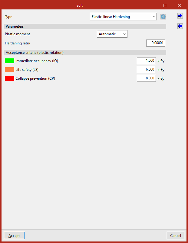
- When selecting "Entered", the hinge data is entered directly into the "Edit" window that appears when you click on the edit button on the right;
- When selecting "From library", you must select a specific type of hinge from those previously defined in the "Plastic hinge library" in the "Project" tab.
The "Export" and "Import" options in the "Edit" window allow you to create plastic hinges types in the library based on the data entered here, as well as to import library data if required.
Editing plastic hinges
Alternatively, if you select "Plastic hinges" in the "Properties - Selection" window, you can select the plastic hinges previously entered in the model and edit their data.
| Note: |
|---|
| Please follow this link to find out about the different types of plastic hinges available. |
Viewing plastic hinges
In the "Forces" view (within the "Analysis" tab), the plastic hinges that have reached the yield point in the selected load case are highlighted by an increase in size and a colour change.
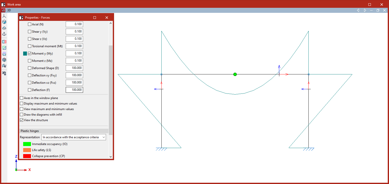
| Note: |
|---|
| Taking plastic hinges into account when analysing a structure requires performing a non-linear analysis using the OpenSees analysis engine. |
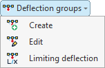
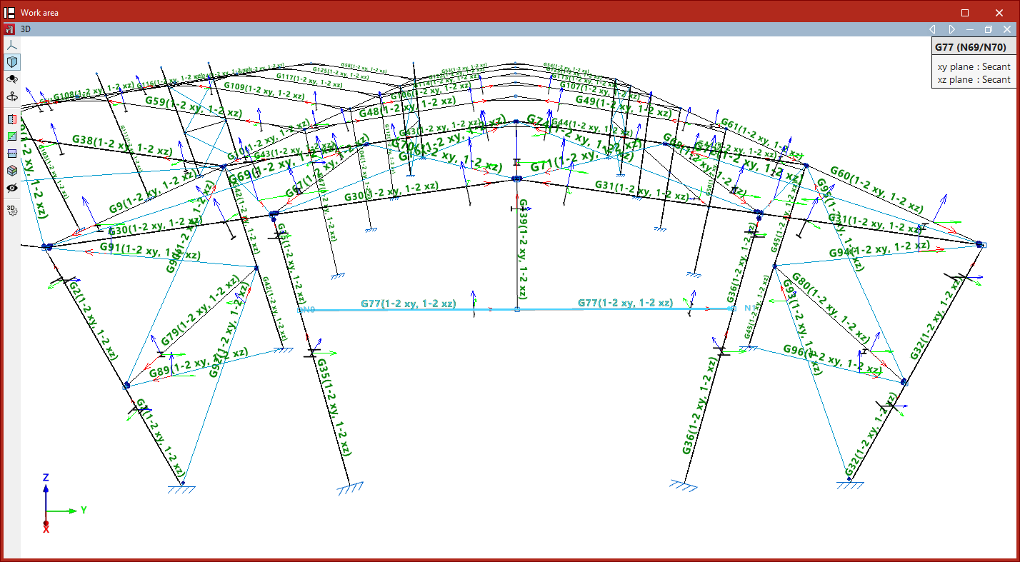
Defining deflection groups and limiting deflection for bars
You can create and edit deflection groups, as well as define the limiting deflection of the beams, using the options in the "Deflection groups" menu, which is available in the "Beams" section of the top toolbar, within the "Properties" tab (under the "Structure" sub-tab).

They are as follows:
- Create
- Edit
- Limiting deflection
Creating deflection groups
First, click on the "Create" option to create deflection groups.
A deflection group is a set of aligned bars that are considered together when calculating deflection, even if there are intermediate nodes.
When this option is selected, the program displays text above the bars indicating the deflection group to which they belong and, in brackets, the type of deflection in each of the two local planes of the section. By default, each bar is a single secant deflection group.
If desired, you can group several aligned bars together to calculate their deflection as a single unit. To do this, left-click on the start node and then on the end node of the group of aligned bars.
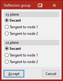
This opens the "Deflection group" window, where you can select the deflection type for each of the two local XY and XZ planes of the section.
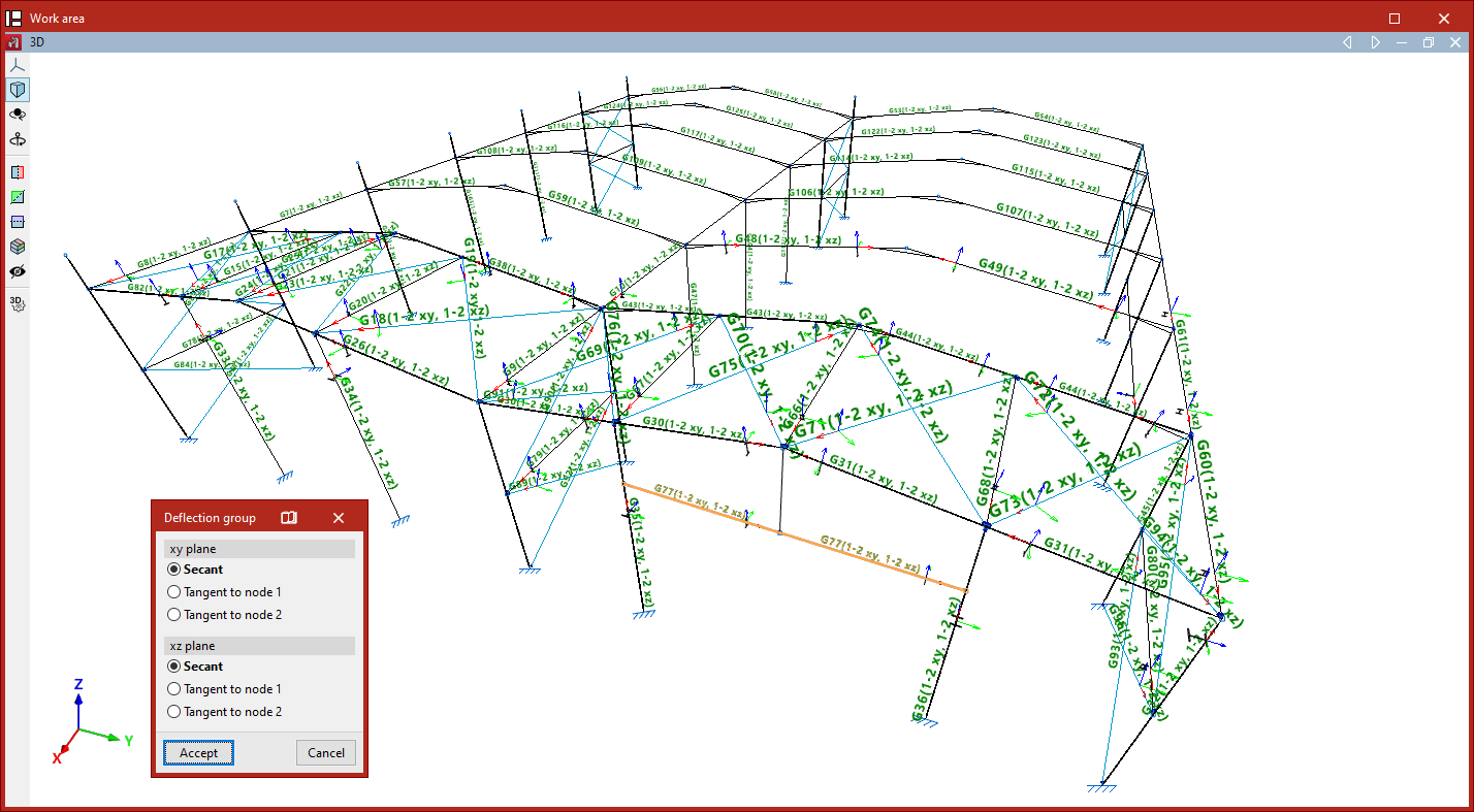
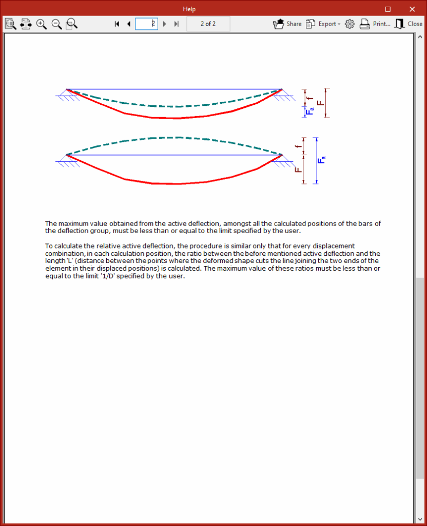
This could be "Secant", "Tangent to node 1" or "Tangent to node 2":
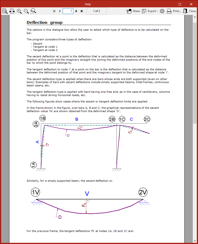
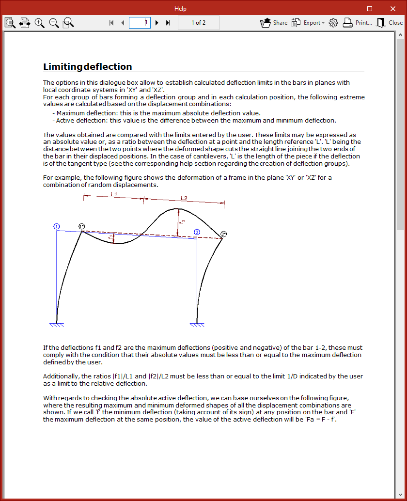
- The secant deflection is defined as the distance between the curved line and the straight line connecting its two endpoints.
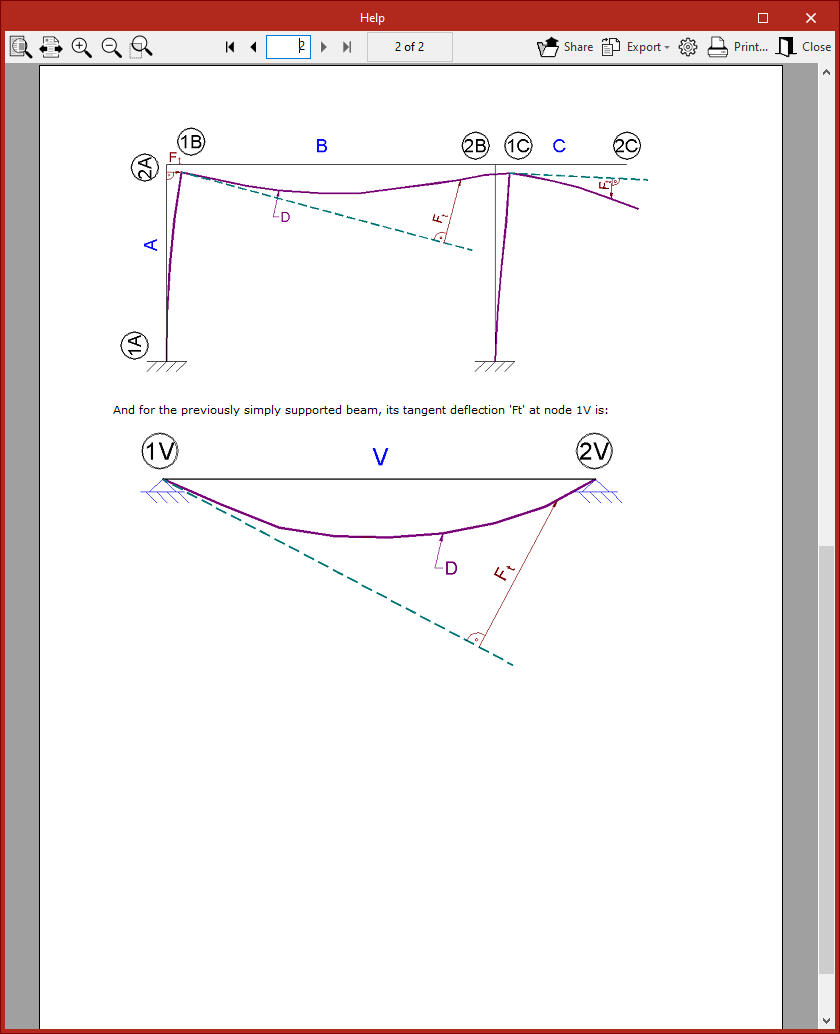
- The tangent deflection, on the other hand, is the distance between the curved line and the straight line tangent to the curved line at one of its endpoints.
| Note: |
|---|
| Typically, the secant deflection is used for interior spans between columns, and the tangent deflection for cantilevers or columns with drifts. |
For more information on calculating deflection, click on the button at the top of the window’s title bar to access the program’s "Help" section.
After clicking "Accept", the program creates the deflection group between the selected nodes.
Editing deflection groups
The next menu option is "Edit", which allows you to change the deflection style of groups that have already been created.
When you hover the cursor over each deflection group, a box appears on the screen displaying the information entered. In addition, the two end nodes are identified in the model.
You can select the groups by clicking on them one by one or by using a selection window. Then, right-click.
This brings up the "Deflection group" window, where you can modify the deflection types selected for each of the section's local planes.
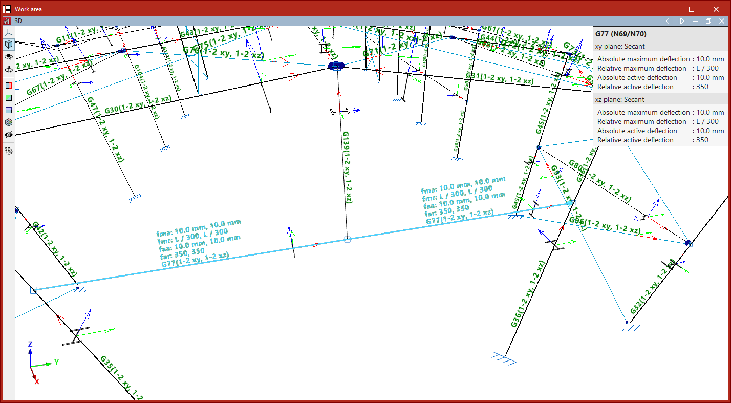
Defining the limiting deflection
Finally, use the "Limiting deflection" option to set the deflection limits for each group. After selecting the groups, right-click to open the settings window.
To make it easier to identify the local section planes, a diagram showing the local coordinate axes is provided at the top; these use the same colour coding as in the model.
You can then tick the various boxes to apply the "Absolute maximum deflection", "Absolute active deflection", "Relative maximum deflection" and "Relative active deflection" to both planes.
Absolute deflection limits are entered in the units of measurement defined in the project, whilst relative deflection limits are specified as a specific fraction of the reference length "L".
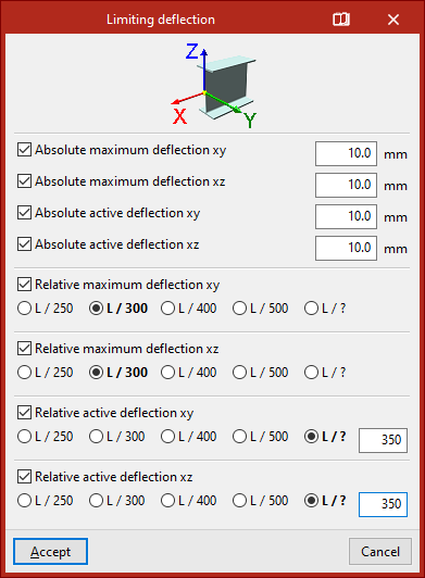
The maximum deflection refers to the maximum deflection in the specified plane for all combinations of displacements.
Furthermore, the active deflection is defined as the difference between the maximum and minimum deflections.
The top button on the title bar of this window allows you to access the program’s “Help” section regarding the definition and calculation of the values mentioned.
After clicking "Accept", the applied limit values will be displayed on the beams in the model and in the tooltip that appears when you hover the cursor over them.
| Note: |
|---|
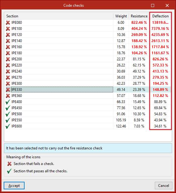
| Next, from the "Analysis" tab, you can use the "Check elements" option to verify whether the sections in the series comply with the specified limit deflection values. |
Fire resistance settings (the "Properties" tab)
To configure the fire resistance of specific bars, select the "Fire resistance" menu from the "Bars" section at the top of the "Properties" tab interface.

The options in this menu will be available if you have previously enabled the fire resistance check in the "General data" section of the "Project" tab.
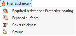
The options available in this menu are as follows:
- Required resistance / Protective coating
- Exposed surfaces
- Cover thickness
- Groups
Each of these features is described below:
Required resistance / Protective coating
The "Required resistance / Protective coating" option allows you to define specific settings for testing the fire resistance of a selection of bars.
After clicking on the option, select the bars one by one using the left mouse button, or highlight a capture area and click the right mouse button.
The "Fire resistance" window then appears. Here, the program displays the type of member selected – in this case, "Steel sections" – and allows you to either "Use the configuration entered in the general data of the job" or "Configure the fire resistance check" specifically.
If the second option is selected, the same options available in the "Fire resistance" settings under "General data" will appear; however, in this case, once "Accept" is clicked, they will apply only to the selected bars.
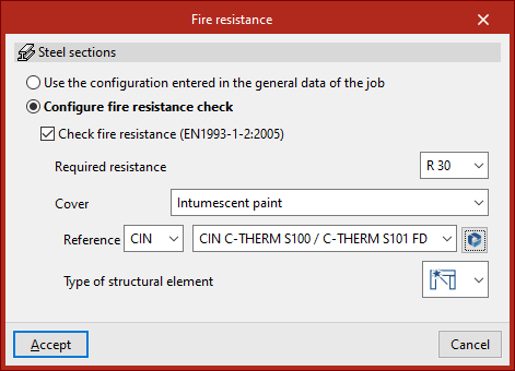
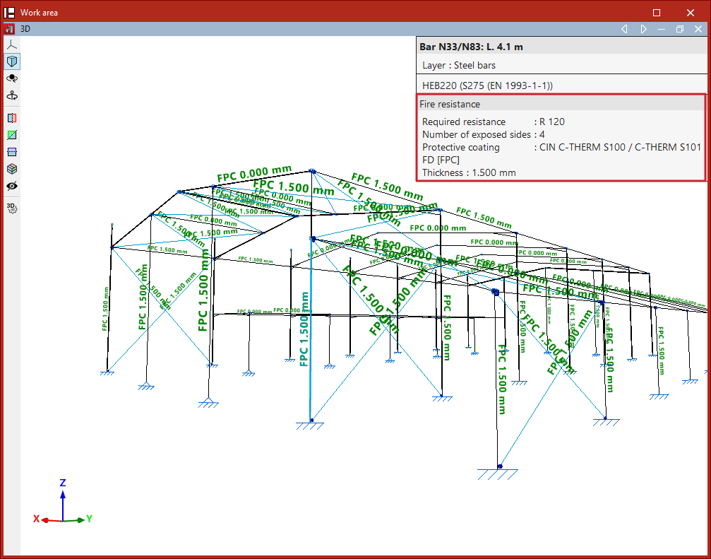
Using this option, you can also hover the cursor over the bars to display an information box specifying the defined "Fire resistance" and, where applicable, the type of protective cladding.
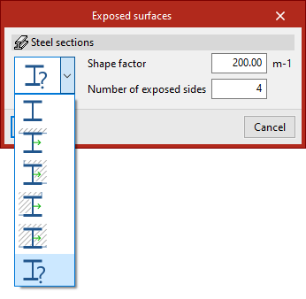
Exposed surfaces
The "Exposed surfaces" option allows you to specify which surfaces of the bars are exposed to fire. This enables you to optimise the thickness of the protective coating, as well as the cross-sections of the bars, where the surfaces of the bars are not exposed to fire.
Definition of exposed surfaces in steel sections
In the "Exposed surfaces" window that appears after selecting the sections, you must select one of the following options from the drop-down menu to define the section’s exposure.
In the first option, the program automatically calculates the shape factor based on the exposed surfaces:
- Section with all four exposed sides
- Section with three exposed sides (side and bottom)
- Section with two exposed sides (right side and bottom)
- Section with exposed sides (left side and bottom)
- Section with one exposed sides (bottom)
By default, and as a conservative approach, the program assumes a section with four exposed faces.
In the last option, the user manually enters the "Shape factor" and the "Number of exposed sides" (between 1 and 4).
| Note: |
|---|
| The program displays the local Y-axis of the section in green on the symbol for each type of exposure, to identify the position and orientation of the exposed surfaces relative to it. |
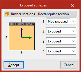
Defining exposed surfaces on timber bars
For timber beams with a rectangular cross-section, you can specify for each of the four surfaces of the cross-section whether it is "Exposed" to fire or "Not exposed".
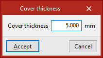
Cover thickness
The "Cover thickness" option allows you to enter the thickness of the fire-retardant coating applied to the selected bars directly.
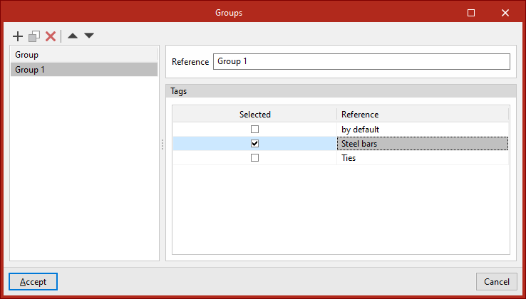
Groups
The program can deisng the thicknesses of fire-resistant cladding. The design can be carried out by setting the thickness of bars belonging to the same group to the same value, among other options. The "Groups" option allows you to create design groups, which can consist of bars assigned to one or more labels.
You must enter a "Reference" for each group and, by ticking the relevant boxes, select the "Labels" assigned to the elements you wish to include in each group.
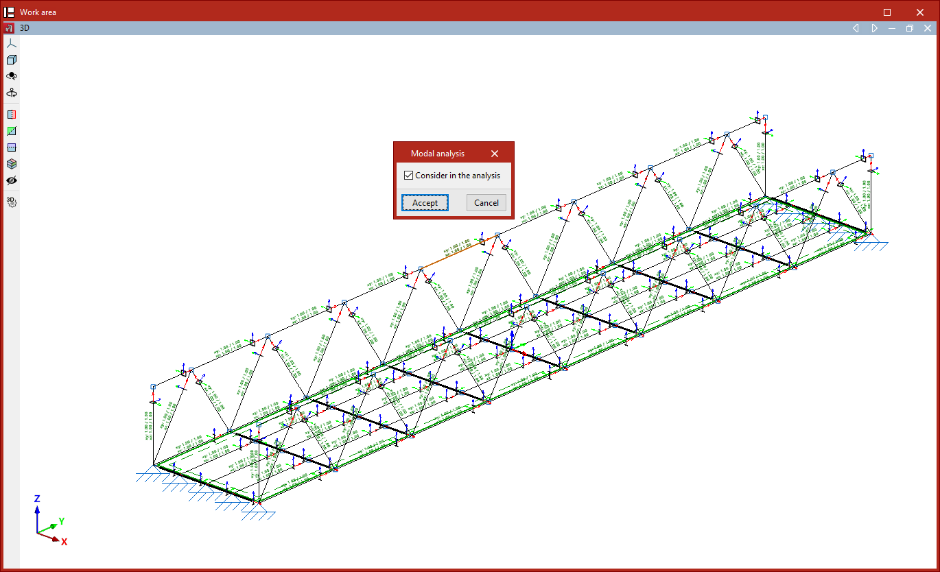
Selecting the bars and shells to be considered in the modal analysis
To perform a modal vibration analysis in the program, you must select the bars and shells to be included in the analysis. To do this, use the following options in the "Properties" tab (under the "Structure" tab).

Modal analysis
The "Modal analysis" option, available in both the "Bars" and "Shells" groups, allows you to include bars and/or shells in the modal vibration analysis carried out by the program.
To do this, select a group of bars and/or shells using the left mouse button and, after clicking the right mouse button, tick the following box in the window that appears:
- Consider in the analysis (optional)
Next, in the "Modal" section, under the "Analysis" tab (also under the "Structure" tab), the remaining steps for configuring, running and viewing the results of the modal analysis will be carried out.
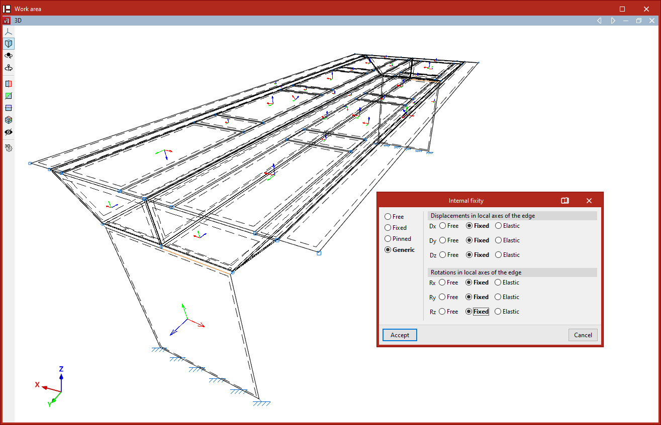
Defining the internal fixity of shells
The definition of internal fixity on shell edges is carried out using the following option, available in the "Shells" group on the top toolbar, within the "Properties" tab (in the "Structure" section).

Internal fixity
The "Internal fixity" option allows you to edit the internal fixity of a group of edges.
Internal fixities define how the shell edges are connected to other adjacent elements present in the model, such as beams or other shells.
To do this, select the edges you wish to edit using the left mouse button or by drawing a selection box, then right-click.
In the pop-up window, you can define whether the internal fixity is "Free", "Fixed", "Pinned", or "Generic". In the latter case, you can specify whether the "Displacements in the local axes of the edge" (Dx, Dy, and Dz) and the "Rotations in the local axes of the edge" (Rx, Ry, and Rz) are free, fixed, or elastic.
Then, click "Accept".
In the model view, the program represents each of these fixities differently.
The internal fixity defined in this way affects the internal nodes of the edge that are generated through the discretisation of the shells. To modify the internal fixity at the end nodes of the edge, you must use the "Internal fixity" option in the "Node" group.
External fixity definition for shells
The definition of external fixities on the edges of shells is carried out using the following option, available in the "Shells" group on the top toolbar, within the "Properties" tab (under the "Structure" section):

External fixity
To edit the external fixities of a group of edges, use the "External fixity" option.
After selecting the option, choose the edges to be edited using the left mouse button or by drawing a selection box, then right-click.
The program will open a window where you can choose the type of external fixity, which will be applied once you click "Accept".
External fixities define the global constraints on the selected edges. They restrict the displacement or rotation of the edge nodes and correspond to supports on the ground or on other external elements in the model.
The defined external fixity affects the internal nodes of the edge created by the discretisation of the shells, as well as the end nodes, if no external fixity has already been defined for them.
If an edge node is shared by edges with different external fixity conditions, none will be applied, and the node will remain unconstrained. The program displays a warning for such conflicting nodes in the "Analysis" tab using the "Show/Hide issues" option.
Free
By default, the edges of a newly introduced shell are defined as "Free", i.e., with no external fixity.
The remaining options allow you to define external fixity on the edge:
Generic
The "Generic" option allows you to manually define constraints on displacements and rotations in all three spatial directions.
Displacements
The displacements can be "Independent", "Along a line" or "On a plane".
For those defined as "Independent", the behaviour of the displacements along the three axes, Dx, Dy, and Dz, is specified:
- Free – the displacement in that direction is unconstrained.
- Fixed – the displacement is constrained to a fixed value (default is zero unless modified by the "Prescribed displacements" option under the "Load" tab).
- Elastic – an elastic support is applied in that direction. You must specify the stiffness constant of the support in the indicated units and its Direction ("Both", "Negative", or "Positive").
For displacements defined as "Along a line", the edge nodes may only move in the direction of a vector defined by its X, Y, and Z components entered on the right. In the perpendicular directions, the support can be specified as "Fixed" or "Elastic".
For displacements defined as "On a plane", the edge nodes may move within a plane perpendicular to a vector defined by the entered X, Y, and Z components. In the direction normal to the plane, the support can be either "Fixed" or "Elastic".
Rotations
For Gx, Gy, and Gz "Rotations", the following can be defined:
- Free – the rotation is unconstrained in that direction.
- Fixed – the rotation is constrained to zero.
- Elastic – an elastic rotational support is applied. You must provide the stiffness constant and specify the Direction ("Both", "Negative", or "Positive").
The remaining options in the "External fixity" panel correspond to predefined fixities that simplify data input and speed up the process:
Fixity
The "Fixity" option fully restrains displacements (Dx, Dy, Dz) and rotations (Gx, Gy, Gz) in all three directions at the nodes of the selected edge.
Each displacement or rotation must be defined as either "Fixed" or "Elastic".
Pinned
The "Pinned" option restrains only the displacements (Dx, Dy, Dz) in all three directions at the nodes of the selected edge, while allowing rotations.
Each restrained displacement must be defined as either "Fixed" or "Elastic".
Free displacements along a line in the X, Y, or Z direction
These options allow free displacements along a line in the global X, Y, or Z directions.
The first row defines fixed supports with free displacement and also restrains rotations:
- Free displacement along the X direction
- Free displacement along the Y direction
- Free displacement along the Z direction
The second row defines pinned supports with free displacement and leaves rotations unconstrained:
- Free displacement along the X direction with unconstrained rotations
- Free displacement along the Y direction with unconstrained rotations
- Free displacement along the Z direction with unconstrained rotations
In all cases, the components of the line’s direction vector are pre-filled in greyed-out numeric fields. The user must specify whether displacement or rotation in each direction is "Fixed" or "Elastic".
Free displacements along an arbitrary line
These options allow free displacement along an arbitrary line, with or without constrained rotations:
- Free displacement along an arbitrary line
- Free displacement along an arbitrary line with unconstrained rotations
In this case, the user enters the components of the direction vector for the line, and specifies for each shown direction whether the displacement or rotation is "Fixed" or "Elastic".
Free displacements on a plane parallel to the XY, XZ, or YZ axes
LThese options define free displacements on a plane parallel to one of the global axes (XY, XZ, or YZ).
The first row defines fixed supports with free displacement and restrained rotations:
- Free displacement on a plane parallel to the XY plane
- Free displacement on a plane parallel to the XZ plane
- Free displacement on a plane parallel to the YZ plane
The second row defines pinned supports with free displacement and unconstrained rotations:
- Free displacement on a plane parallel to the XY plane with unconstrained rotations
- Free displacement on a plane parallel to the XZ plane with unconstrained rotations
- Free displacement on a plane parallel to the YZ plane with unconstrained rotations
In all these cases, the components of the plane’s normal vector are pre-filled in greyed-out numeric fields. The user simply indicates whether displacement or rotation in each shown direction is "Fixed" or "Elastic".
Free displacements on an arbitrary plane
Finally, it is possible to define free displacement on an arbitrary plane, either with constrained or unconstrained rotations:
- Free displacement on an arbitrary plane
- Free displacement on an arbitrary plane with unconstrained rotations
You must enter the components of the plane’s normal vector and specify whether displacement or rotation in each shown direction is "Fixed" or "Elastic".
Inserting and editing force integration strips in shells
Force integration strips can be added and edited in shells using the "Integration strips" option, which is available in the "Shells" section of the top toolbar, within the "Properties" tab (under the "Structure" sub-tab).

The integration strips in the plates define lines along which, for a given bandwidth, the forces corresponding to the plate are integrated to obtain the bar forces.
Integration strips
After clicking on the option, select the slides using the left mouse button or by dragging to select a capture area, then click the right mouse button to confirm.
The geometry of the first selected sheet is displayed in the centre of the pop-up window. If more than one shell has been selected, once editing is complete, the integration strips are copied to the remaining selected shells.
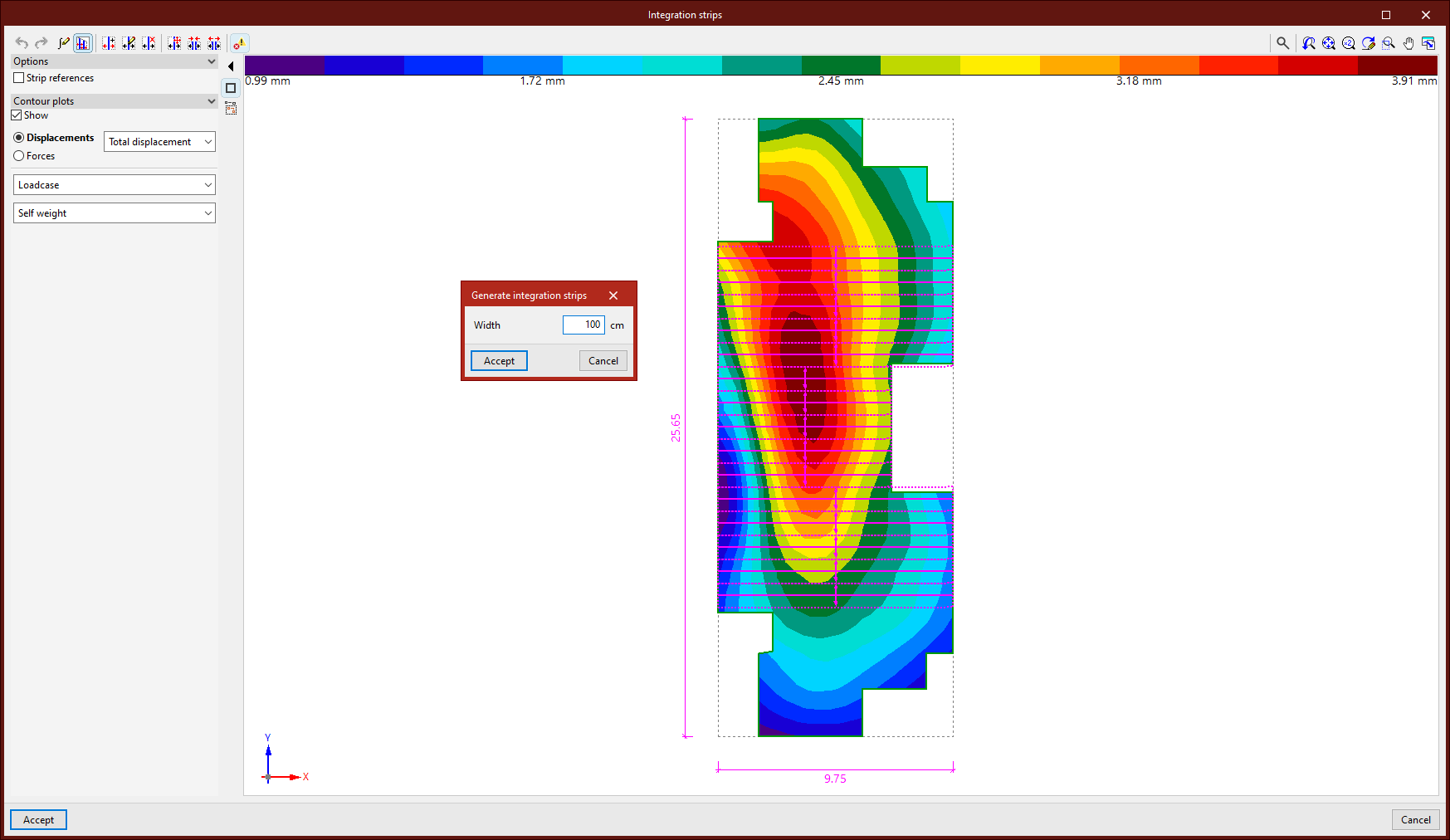
Display options
On the left-hand side, the program allows you to display the "Strip references" once they have been entered, as well as the "Contour plots" for "Displacements" and "Forces" if the structure has been analysed. You can also enable "Screenshots" here.
Configuring the integration of forces in strips
The first button on the top toolbar allows you to define the "Integration of forces in strips". This can be set to "Based on the internal forces", in which case you can "Use smoothed forces" by ticking the relevant box, or "Based on the nodal forces". A detailed explanation of these methods can be found in the "Help" section, which can be accessed by clicking the button on the title bar of this window.
Generating integration strips
The following button allows you to "Generate integration strips in the zone". First, enter the "Width" of the strips. Then, after clicking "Accept", use the left mouse button to select four points that define the generation area. The integration strips are parallel to the line defined by the first two points selected and will be generated within the zone, taking into account the geometry of the sheet.
Issues
The last option on the top toolbar allows you to "Show/Hide issues" for elements where an error has occurred. If you hover the cursor over these elements, the program displays a message describing the error.
Introduction and manual editing of integration strips
The other options on the top toolbar allow you to enter and edit integration strips manually:
- Use the "New" option to insert a new integration strip. To do this, after entering the "Width" and clicking "Accept", select two points on the image using the left mouse button.
- From the "Edit" menu, you can modify the properties of several integration strips simultaneously. To do this, select the strips using the left mouse button or highlight a capture area, then right-click. In the pop-up window, adjust the "Width" and the "Number of force points".
- Use this option to "Delete" a group of integration strips. Similarly, select the strips using the left mouse button or by dragging to create a selection area, then click the right mouse button to confirm.
- The "Move end" function moves the end of an integration strip. To do this, left-click to select the end of the band, and then select its new position.
- It is also possible to "Join" several integration strips. After clicking on the option, select several parallel strips using the left mouse button or by dragging to define a selection area, then confirm with the right mouse button. This creates a single integration band within the area defined by the selected bands.
- To "Divide" multiple integration strips, click on the relevant option and then select the strips using the left mouse button or by dragging to select an area. Right-click, enter the "Number of divisions" in the dialog box, and click "Accept". Multiple integration strips will be generated in place of each selected strip.
To finish editing the integration strips and confirm the changes, click "Accept".
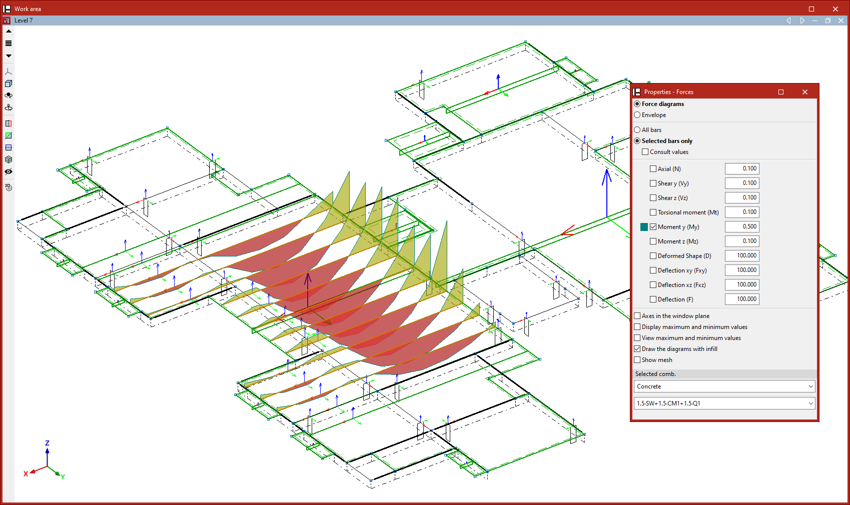
Checking forces in integration strips
Creating integration strips allows you to view the forces in each strip as if they were the forces acting on a structural beam.
To do this, once the structural analysis has been carried out, use the "Forces" option in the "Stress / Strain" group on the "Analysis" tab.
Editing shell properties
The following tools for editing shell properties are available in the "Shells" section of the top toolbar, within the "Properties" tab (under the "Structure" sub-tab).

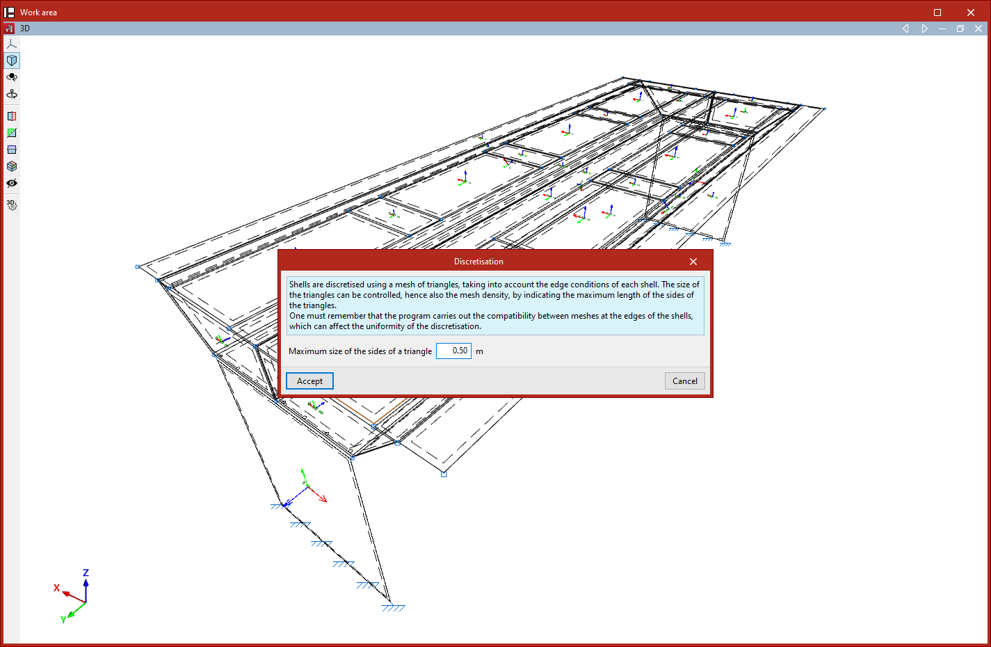
Discretisation
The shells are discretised using a triangular mesh; furthermore, the program considers the boundary conditions for each plate.
The "Discretisation" option allows you to control the design of these triangles and, consequently, the mesh density. To do this, select the group of shells using the left mouse button or by dragging to select an area, and then right-click.
In the window that appears, the maximum dimension for the sides of the triangles is specified in the following field:
- Maximum size of the sides of a triangle
Changing the mesh density affects the computation time and may alter the results obtained.
| Note: |
|---|
| The program performs mesh matching at the edges of the elements, which may affect the uniformity of the discretisation. |
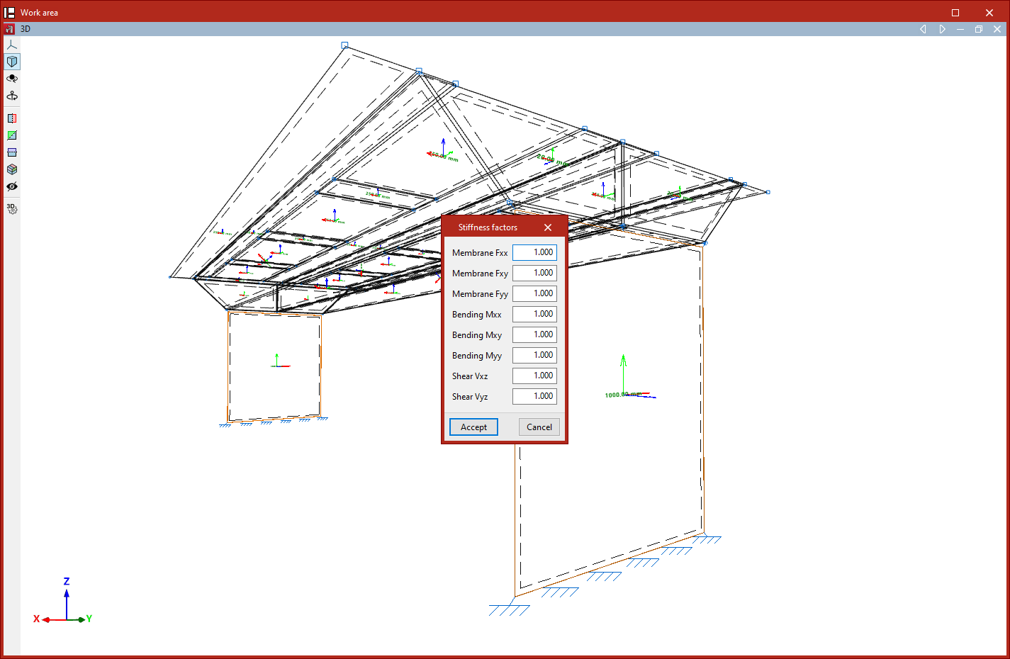
Stiffness factors
The "Stiffness factors" option allows you to define stiffness modification factors for a group of plates. To do this, select the plates using the left mouse button or by dragging a selection area, and then right-click.
In the window that appears, you can use these factors to modify the axial, shear and bending stiffness along the different local axes of the plate:
- Membrane Fxx
- Membrane Fxy
- Membrane Fyy
- Bending Mxx
- Bending Mxy
- Shear Vxz
- Shear Vyz
By default, the scaling factors are set to 1 in all cases.
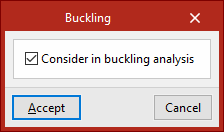
Buckling
This option allows you to include shells in the buckling analysis carried out from the "Analysis" tab.
To do this, select a group of shells using the left mouse button and, after clicking the right mouse button, tick the following box in the window that appears:
- Consider in buckling analysis (optional)
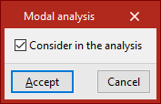
Modal analysis
This option allows you to include shells in the modal vibration analysis performed via the "Analysis" tab.
To do this, select a group of shells using the left mouse button and, after clicking the right mouse button, tick the following box in the window that appears:
- Include in the analysis (optional)
Inserting elements with non-linear behaviour
As well as designing structures using linear analysis, in which all elements have an exclusively linear behaviour, the program allows you to include elements with non-linear behaviour and perform non-linear analysis.
The elements for which a non-linear analysis can be performed are as follows.
Bars only in tension and compression-only bars
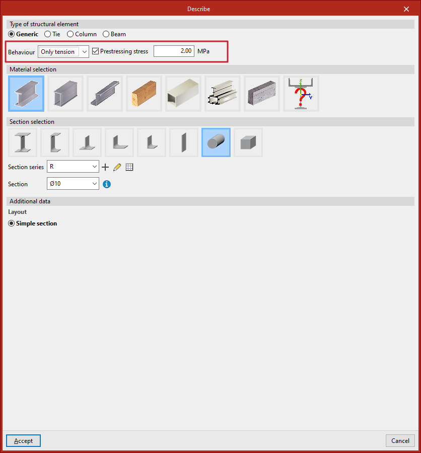
To model a beam subjected only to tension or only to compression, in the "Describe" window that appears when editing its cross-section, you must enter a "Generic" beam type and, under the "Behaviour" option, select either "Only tension" or "Only compression".
Optionally, you can enter a "Prestressing stress" for bars designed for tensile behaviour only from this panel.
Uplift at supports
The program allows you to define the non-linearity of the supports for two types of elements:
- For nodes or edges of shells defined using "External fixity", you can specify whether the "Direction" of the elastic constraint for each constrained degree of freedom is "Positive", "Negative" or "Both".
- In sheets with a "Subgrade modulus in the local Z axis", you can specify whether the "Behaviour" is "Linear" or "Only compression".
If the elastic restraint acts in a single direction, or if the shell is assumed to behave as a pure compression member, it is possible to consider the occurrence of uplifts at those supports.
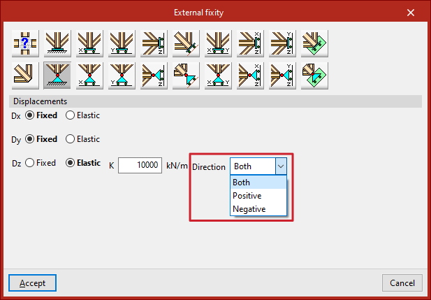
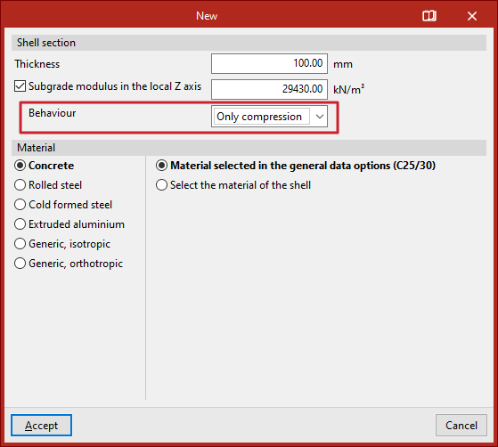
Table of contents
Complete your CYPE 3D journey by exploring the other available sections:
- Introduction
- Start: creating new projects, workflows, and examples
- Setting the work environment
- Setting the job data
- Defining the structure’s geometry
- Editing the properties of structural elements
- Entering and editing loads on the structure
- Designing and analysing connections
- Analyses, checks, and results
- Defining and editing reinforcement
- Designing and analysing foundation
- Printing documents and exporting data