
Introduction
Pushover analysis can be used to realistically evaluate the non-linear response of a structure subjected to seismic forces through the incremental application of lateral loads under displacement control.
This procedure can be used to:
- Study the seismic behaviour of the building, identifying the sequence of plastic hinge formation and the potential mechanisms of collapse.
- Identify structural deficiencies and areas of concentrated damage, thereby facilitating the design and assessment of reinforcement measures.
- Determine the structure's capacity curve and identify its performance point.
- Assess new-build structures during the design stage, as well as existing structures for seismic assessment, rehabilitation, or strengthening.
CYPE 3D can be used to perform a pushover analysis on a structure entered into the program, using the options in the "Pushover" group on the "Analysis" tab.
Workflow for carrying out a pushover analysis on a structure
Prerequisites
Pushover analysis is a second-stage analysis. The structure must have been previously designed using the results of the linear analysis and must satisfy all the necessary checks and requirements.
When it comes to connections, they should be designed so that the failure mechanism occurs in the beams or columns rather than in the connection itself. Pre-qualified connections, for example, meet this requirement by definition.
Modelling
Once the structure has been entered and designed in accordance with the considerations mentioned above, the pushover analysis can then be modelled using the following workflow:
- Defining the non-linearities to be taken into account:
- Creating plastic joint types (from the "Plastic hinge library" in the "Project" tab).
- Assigning plastic ball joints to the bars (from "Plastic hinges" in the "Properties" tab).
- Defining loadcases for pushover analysis (under "Loadcases" in the "Pushover" section of the "Analysis" tab), including the definition of the initial load condition, the control node and the lateral load patterns.
- Performing the pushover analysis (from "Analyse", in the "Pushover" section of the "Analysis" tab).
- Reviewing pushover analysis results (from the other options in the "Pushover" section of the "Analysis" tab: "Displacements", "Reactions", "Forces", "Contour plots", "Capacity", "Plastic hinges").
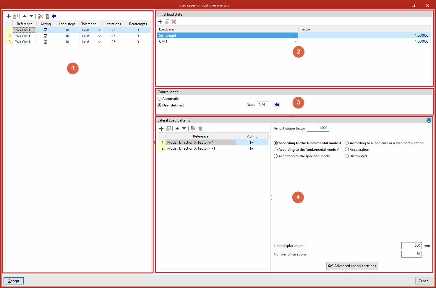
Defining load cases for the pushover analysis
Load cases for pushover analysis are created and edited using the "Load cases" option, available in the "Pushover" section of the top bar, within the "Analysis" tab (under the "Structure" sub-tab):

For each load case in the list (1), the following is defined:
- the "Initial load state" (2),
- the "Control node" (3),
- and the "Lateral load patterns" (4).
Load cases
The "Load cases" option is used to define the load cases for the pushover analysis.
Clicking this opens the "Load cases for pushover analysis" window. These load cases must be added to the list on the left-hand side using the options on the top toolbar. Each load case is defined as follows:
- The "Reference" is generated automatically based on the load cases and combination factors defined below.
- Indicate whether the case is "Acting" or not by ticking the relevant box.
- Several "Load steps" are defined, the "Tolerance" value is selected, and the number of "Iterations" used in the analysis and the number of "Reattempts" are entered.
Alternatively, you can also click the assistant button at the top of the load case list to "Import the load cases defined for the modal analysis".
Initial load status
Next, in the top-right-hand corner, the "Initial load state" is defined for each load case selected from the list.
To do this, add entries to the list by selecting "Loadcase" from the drop-down menu and entering the value for "Factor" for each one.
Control node
The "Control node" section allows you to define the control node for each load case selected from the list in two ways:
- "Automatic", in which case the program will select a node located at the highest point of the structure, as close as possible to the geometric centre of that area, and whose degrees of freedom Dx and Dy are not constrained.
- or "User defined", in which case you must either enter the node reference directly or click the "Available nodes" button to select it from the list.
Lateral load patterns
For each selected load case, you must define the list of "Lateral load patterns" in the bottom right-hand corner.
Each load pattern must be entered into the pattern list, which displays its "Reference" (generated automatically) and allows you to specify whether it is "Active" or not.
Next, on the right-hand side, for each pattern, enter the "amplification factor" and select the lateral load distribution (FEMA 356, 3.3.3.2.3) from the following options (lateral loads will be applied to the mathematical model in proportion to the distribution of inertia forces):
- According to the fundamental mode X
A vertical lateral load distribution proportional to the shape of the fundamental mode in the X-direction will be applied. The "Limit displacement" and "Number of iterations" are specified.
- According to the fundamental mode Y
A vertical lateral load distribution proportional to the shape of the fundamental mode in the Y-direction will
be applied. The "Limit displacement" and "Number of iterations" are specified.
- According to the indicated moded
A vertical lateral load distribution proportional to the shape of the mode selected from the drop-down menu will be applied in the specified direction. Select the mode, specify the "Limit displacement" and the "Number of iterations", and select the "Monitored displacement" (Dx or Dy).
- Based on a loadcase or a load combination
The selected load combination will be applied as a lateral load distribution. The load combination is defined by entering assumptions and combination factors in a specific list, specifying the "Limit displacement" and the "Number of iterations", and selecting the "Monitored displacement" (Dx or Dy).
- Acceleration
A uniform distribution of lateral forces will be applied at each node, proportional to the node mass. Enter the "Acceleration" value, specify the "Limit displacement" and the "Number of iterations", and select the "Monitored displacement" (Dx or Dy).
- Distributed
A vertical distribution of lateral load proportional to the Cvx values (vertical distribution factor) will be applied. Select the "Type" of distribution from the following options, specify the "Limit displacement" and the "Number of iterations", and select the "Monitored displacement" (Dx or Dy):- Uniformly
In this particular formulation, the exponent 'k' is set to 0. - Triangular
The exponent 'k' is set to 1. - Parabolic
The exponent 'k' is set to 2.
- Uniformly
At the bottom of the page, you can access the "Advanced scan settings" for Pushover by clicking the relevant button.
Advanced settings for pushover analysis
The advanced settings for the pushover analysis can be modified for each lateral load pattern via the "Load cases" option, which is available in the "Pushover analysis" group on the top toolbar, within the "Analysis" tab (under the "Structure" sub-tab):
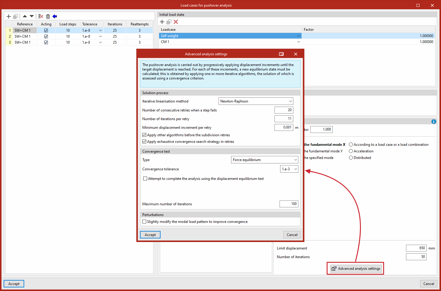
Convergence strategy
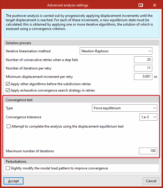
The pushover analysis is carried out by progressively applying displacement increments until the target displacement is reached. For each of these increments, a new equilibrium state must be calculated; this is obtained by applying one or more iterative algorithms, the solution of which is assessed using a convergence criterion.
Given the iterative nature of the solution strategy, the choice of iteration algorithm and the convergence test determines the convergence path of the analysis. Different models or even different directions of analysis may require different strategies; it may even be necessary to modify the strategy at a specific stage of the process.
The pushover analysis algorithm used by the program attempts to reach the target displacement using the user-defined iterative linearisation method. If the convergence test is not satisfied at any stage of the analysis, the algorithm may switch to other secondary methods and/or subdivide the increment size.
Resolution process
The section entitled "Solution process" begins by defining the "Iterative linearisation method". The iterative linearisation method controls how iteration is performed within a load step to satisfy the equilibrium relationship R(u) = Fe - Fi(u) = 0. The available methods are:
- Newton-Raphson
This method is suitable for small or medium-sized models (< 100,000 degrees of freedom (DOFs)). It is the most conservative method. It minimises the residual between iterations because it performs factorisation of the system’s tangent matrix at each iteration, which allows the analysis to progress more accurately when many steps are chained together or the system has a response that is highly sensitive to small perturbations. However, performing the factorisation at each iteration makes it slower than other methods and, at the same time, more sensitive to oscillations.
- Modified Newton-Raphson
This method is suitable for large models (> 100,000 degrees of freedom (DOFs)). It performs the factorisation of the system’s tangent matrix only at the start of the step and thereafter works with an approximation, which makes it faster than the Newton-Raphson method and stable against oscillations. It has linear convergence.
- Krylov-Newton
This method is suitable for large models (> 100,000 degrees of freedom (DOFs)). It factors the tangent matrix at the start of the step and uses the previous residuals to correct the direction of the displacement. It is very robust when the tangent matrix is ill-conditioned.
- Newton-Raphson (linear search, step size 0.5)
- Newton-Raphson (linear search, factor 0.8)
These methods are suitable for small or medium-sized models (< 100,000 degrees of freedom (DOFs)). They work in the same way as the Newton-Raphson method, but in this case, a search is performed in the direction of the displacement increment vector to minimise the residual. This is useful when the Newton-Raphson method oscillates without converging.
For any method, the following must be specified:
- The "Number of consecutive retries when a step fails".
- The "Number of iterations per retry".
- The "Minimum offset increase per retry".
You can also tick the relevant boxes for "Apply other algorithms before subdivision retries" and/or "Apply an exhaustive convergence search strategy during retries".
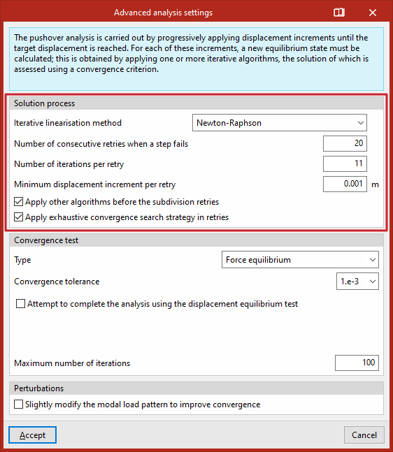
Convergence test
The convergence test calculates the Euclidean norm of the estimated parameter, taking into account all the degrees of freedom in the model. It is used to determine whether the iterative linearisation method has reached an approximate equilibrium within the specified tolerance range.
In the "Convergence test" section, you can define the "Type" by selecting one of the following:
- Balance of forces
This test is usually sufficient to ensure the overall accuracy of the solution obtained. If selected, the program checks that the change in displacement between iterations is less than the specified tolerance. This test uses a single tolerance for the degrees of freedom of translation and rotation. The internal units used are metres and radians.- When selecting this test, you must choose the "Convergence tolerance" from the available options. The "Attempt to complete the analysis using the displacement equilibrium test" option is also available (for which you must select the "Convergence tolerance (displacements)" and enter the "Step subdivision factor").
- Displacement equilibrium
If this test is selected, the program checks that the residual force between iterations is less than the specified tolerance. The internal units used are tonnes. This test is recommended in situations where displacement equilibrium is reached before force equilibrium, which is usually reflected in an irregular displacement-shear force curve and significant variation in forces and moments.- When selecting this test, you must choose the "Convergence tolerance" from the available options.
- Balance of forces and displacements
If this test is selected, the program checks that both the balance of forces and the balance of displacements are satisfied. The results are as accurate as possible, but it can be difficult to get the model to achieve the target displacement.- When selecting this test, you must select the "Convergence tolerance (forces)" and the "Convergence tolerance (displacements)".
- Balance of forces or displacements
If this test is selected, the programme checks that the balance of forces or the balance of displacements is satisfied. It should only be used as a test to analyse model convergence issues.- When selecting this test, you must select the "Convergence tolerance (forces)" and the "Convergence tolerance (displacements)".
- Energy balance
This test should be used as a last resort. If this test is selected, the program checks that the change in energy between iterations is less than the specified tolerance. The tolerance is expressed in units of energy (tonnes × metres in this case). In some deformation modes, this test may return a false equilibrium (when the displacement increment vector is orthogonal to the residual vector).- When this test is selected, the "Convergence tolerance" is selected; the option "Attempt to complete the analysis using the displacement equilibrium test" is offered (for which the "Convergence tolerance (displacements)" is selected and the "Step subdivision factor" is entered).
In addition, the "Maximum number of iterations" is entered for each test.
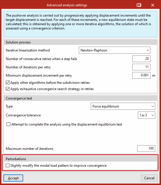
Disturbances
Finally, in the "Disturbances" section, you can tick the relevant box to "Slightly modify the modal load pattern to improve convergence".
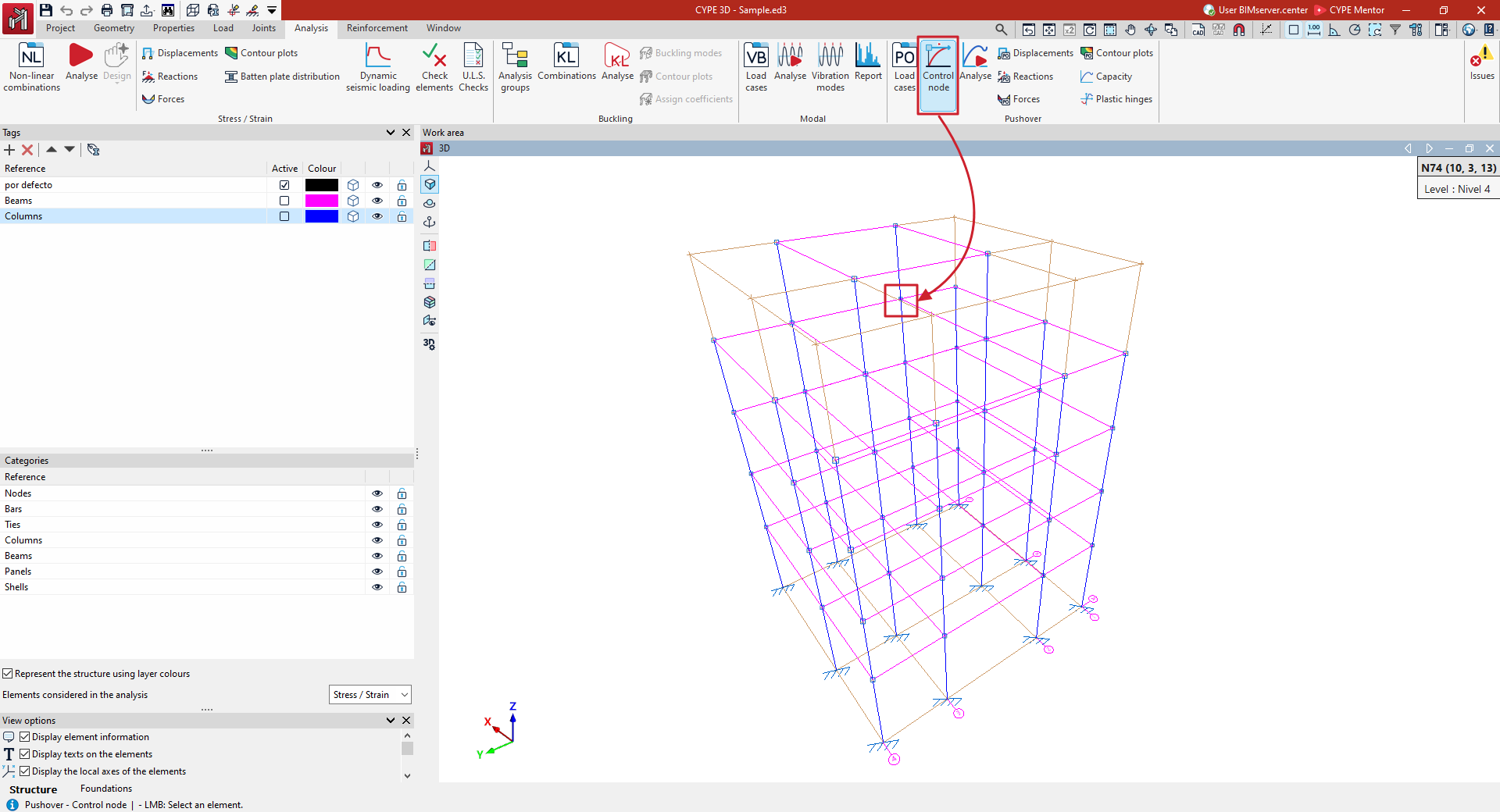
Selecting the control node for pushover analysis
The control node for the pushover analysis is selected using the "Control node" option, available in the "Pushover analysis" group on the top toolbar, within the "Analysis" tab (under the "Structure" tab):

Control node
This allows you to select a node in the structure and assign it as the control node for all load cases in the pushover analysis.
The selected node can be viewed under the "Load cases" option, in the "Control node" section. From here, you can also allow the program to select a control node automatically or specify a control node for each load case.
| Note: |
|---|
| The control node should be located close to the geometric centre of the structure’s highest representative floor. The degrees of freedom Dx and Dy must not be constrained. |
Pushover analysis: "Analyse" option
The following option is available in the "Pushover" section of the top toolbar, within the "Analysis" tab (under the "Structure" tab):

Analyse
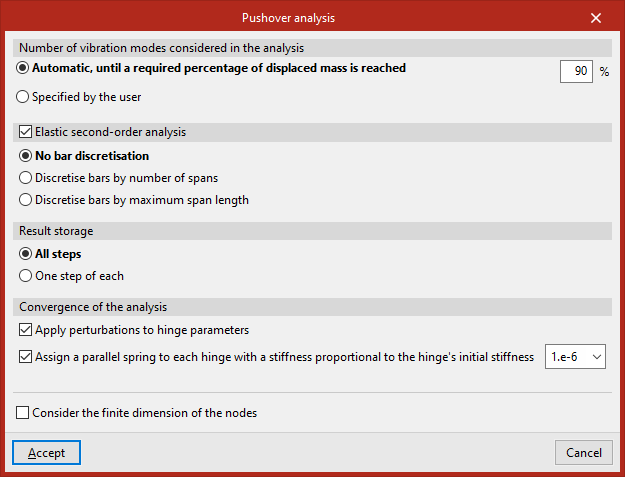
This option can be used to configure and run the pushover analysis.
The "Number of vibration modes included in the analysis" can be:
- "Automatic, until a required percentage of the mass has been displaced", which must be entered.
- "User-defined", in which case the number of modes is entered.
You can then enable "Second-order elastic analysis".
"Result storage" can be carried out:
- For "All loads".
- For"One load in every…", enter a specific number in the box that appears on the right.
Among the options for achieving the "Convergence of the analysis", the program offers the following options:
- Apply perturbations to hinge parameters (optional)
This option can be enabled if the model exhibits convergence issues that prevent the target displacement from being reached. If enabled, the program randomly modifies the yield moment of the hinges by a factor of around 1 in 1000 to try to prevent several hinges from yielding simultaneously, which would trigger a mechanism. - Assign a parallel spring to each ball joint with a stiffness proportional to the ball joint’s initial stiffness (optional)
If the analysis stops because the hinges have collapsed prematurely or the minimum desired displacement has not been reached, this option can be activated to enter springs in parallel with the hinges with very low stiffness in an attempt to ensure that, when they collapse, the system matrix remains invertible.
Finally, you can "Consider the finite dimension of the nodes" by ticking the relevant box.
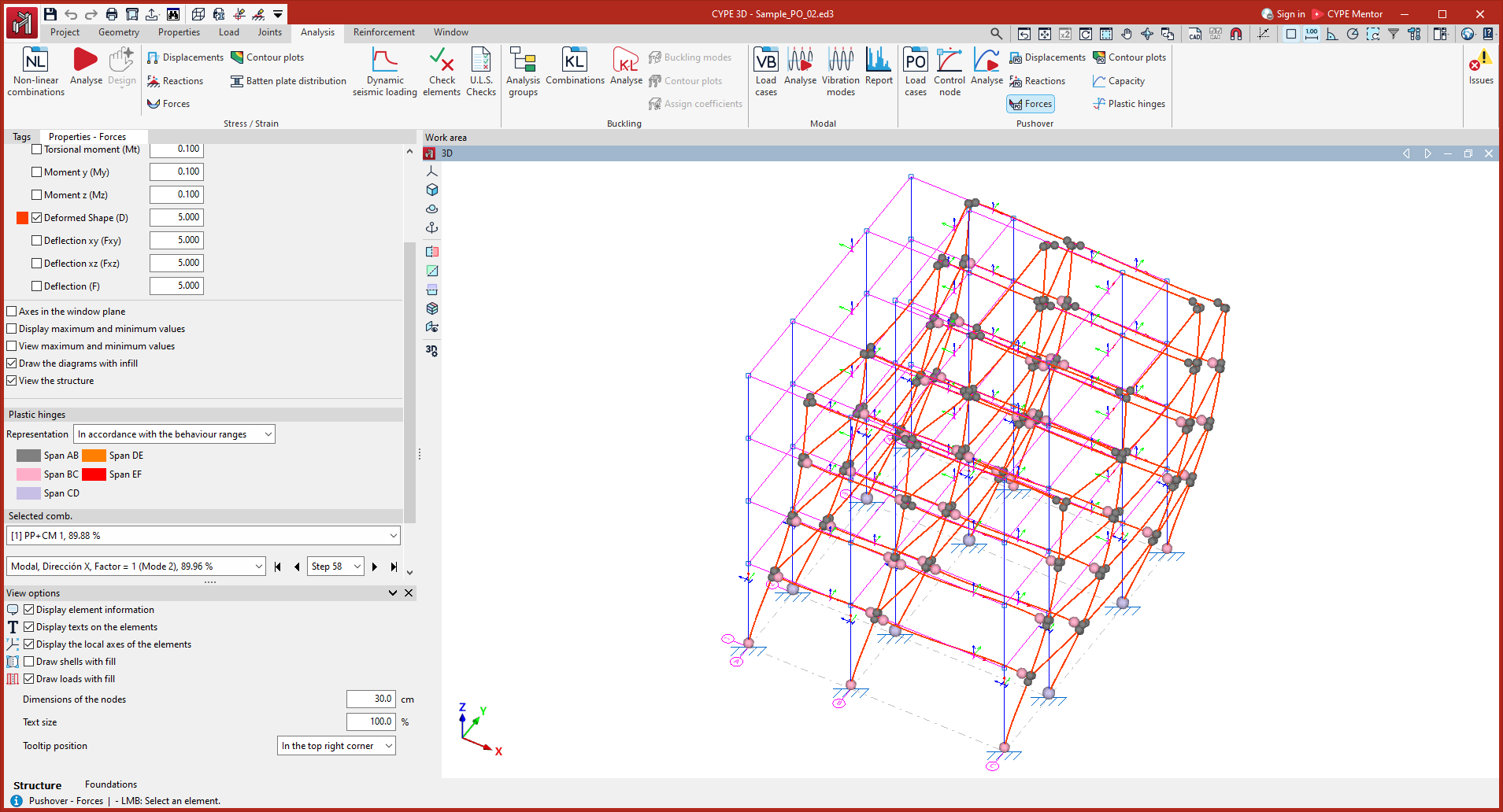
Viewing the forces obtained from the pushover analysis
The forces obtained from the pushover analysis can be viewed using the following option, available in the "Stress / Strain" group on the top toolbar, within the "Analysis" tab (under the "Structure" section).

This tool is similar to the one available for viewing force values following a "Stress/Strain" analysis, but with additional features.
Forces
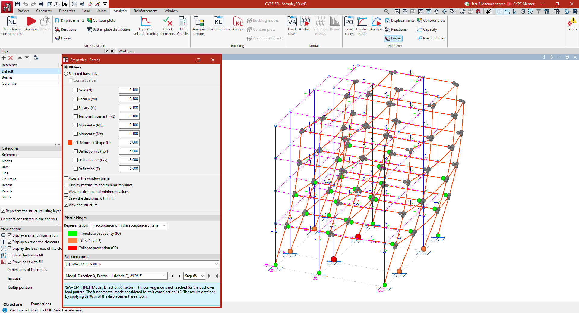
The "Forces" option allows you to plot force diagrams—both normal and shear—on screen for both the bars and the integration bands of the plates, for each step of the pushover analysis.
Selecting forces
In the "Properties - Forces" dialogue box that appears, you can configure the following options.
First, select the bars you wish to view:
- If "All bars" is selected, the graphs for the selected forces will be plotted for all bars in the structure.
- If you tick "Selected bars only", you will need to click on each bar individually for the force plots to be drawn.
- If you tick the "Show values" box, you can hover the mouse cursor over the bars to display an information box showing the values calculated at that point.
The following metrics can be viewed by ticking the boxes in the central section of the dialogue box:
- The "Axial" force.
- The shear force in both directions ("Y-cutter", "X-cutter").
- The "Torsional moment"
- The bending moment in both directions ("Moment y" and "Moment z").
- The "Deformed shape" part of the structure.
- The "Deflection xy" and the "Deflection xz", which correspond to the two planes of the section.
- The total combined "Deflection".
Each graph is displayed in a different colour. This makes it easier to distinguish between graphs on the screen when several are active at the same time.
In addition, to the right of each parameter, you can adjust the scale factor to change the size of the graph display in the viewer.
Other configuration options
Further down, you will find the following options for configuring the display of stress laws:
- The "Axes in the window plane" option displays the stress plots in a coordinate system with the axes drawn on the window plane. This can be useful for making the plots visible in certain views.
- The "Plot maximum and minimum values" option adds information about the maximum and minimum values reached, as well as their positions, to each graph.
- Finally, if only one graph is active, you can select "Show maximum and minimum values". In this case, you must hover the mouse cursor over the bars for the programme to display the maximum and minimum values for each one.
- You can also configure the stress curves to be displayed as filled shapes by ticking the "Draw curves with fill" box.
- Finally, the "View the structure" option allows you to display the structure on screen in its original position.
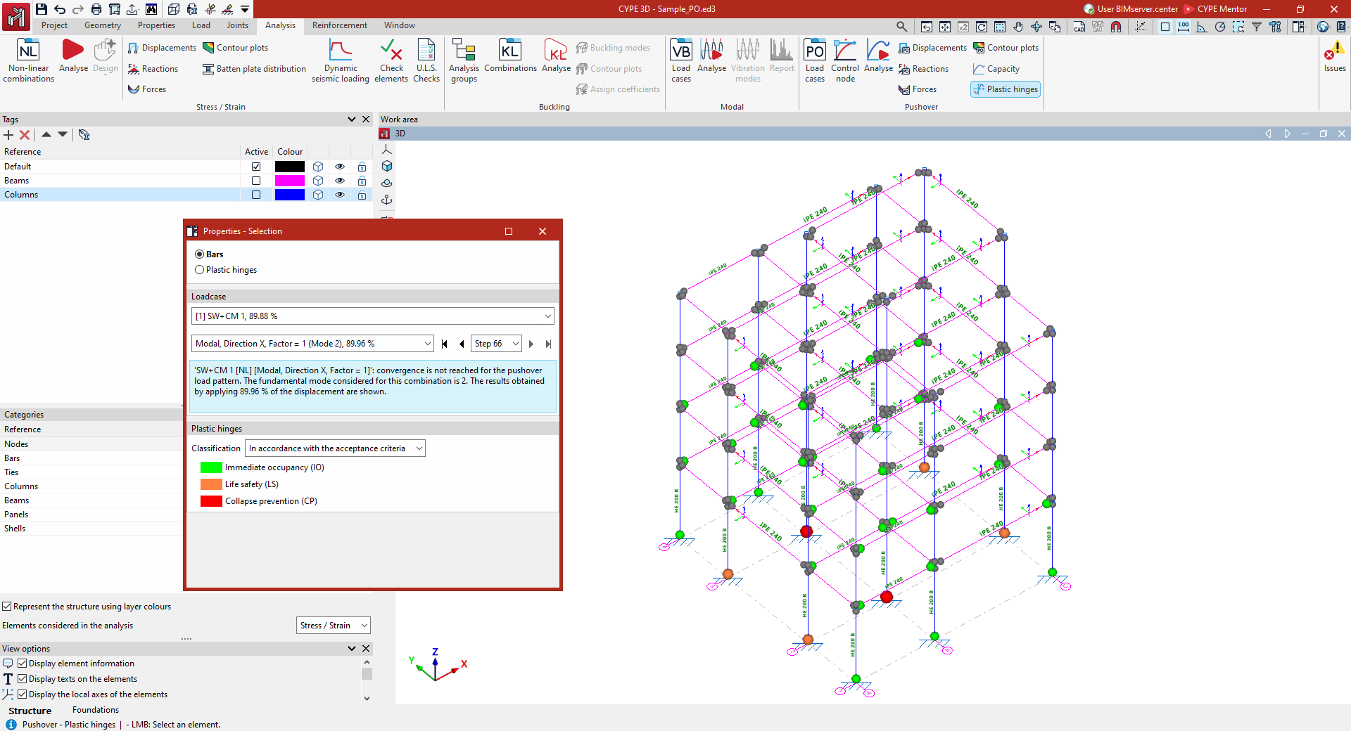
Plastic hinges
In the "Plastic hinges" panel, you can define the "Classification" of the hinges by selecting one of the following options:
- "According to the acceptance criteria" ("Immediate occupancy (IO)", "Life safety (LS)", "Collapse prevention (CP)"); additionally, the ball joint can be found under "Elastic behaviour (shown in grey).
- Or "according to the performance zones" of the ball joints ("Zone AB", "Zone BC", "Zone CD", "Zone DE", "Zone EF").
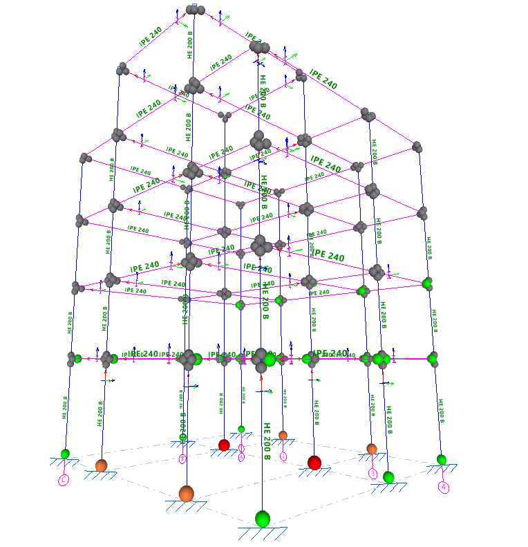
In this way, the hinges will be represented as coloured spheres in the "Work area", scaled according to their state based on the defined classification and the selected load case, load pattern and load step, thereby enabling the behaviour of the structure to be analysed and potential failure mechanisms to be identified.
Selected combination
The results obtained for the load case and lateral load pattern selected from the drop-down menus in the "Selected Comb." panel will be displayed.
On the label of the load case and/or load pattern, the fundamental mode considered is shown in brackets, whilst the percentage value indicates that the results shown have been obtained by applying that percentage of the target displacement.
In addition, in this panel, you can select a specific level from the drop-down menu or navigate between levels using the various buttons provided.
This panel also displays a warning if convergence is not achieved for the selected load pattern.
If the target displacement is reached, the "Limit displacement" value is displayed, the "Monitored displacement" (Dx or Dy) is indicated, and the "Control node" reference is shown.
| Note: |
|---|
| The settings defined in the "Selected Comb." and "Plastic hinge" panels are shared with the other options for viewing pushover analysis results and are synchronised across them. In this way, the settings defined when viewing specific results upon accessing one option (for example, the display of results for a specific step) are retained when accessing another related option. |
Checking the capacity curve and the performance point
The capacity curve and performance point obtained following the pushover analysis can be viewed using the "Capacity" option, available in the "Pushover analysis" group on the top toolbar, within the "Analyse" tab (under the "Structure" sub-tab):

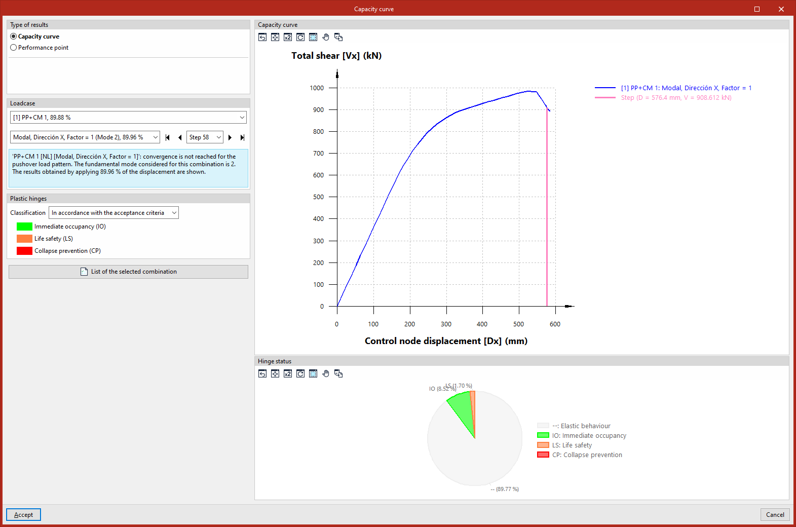
Clicking on this option opens the "Capacity curve" window. Here, under "Result type", you can select whether you wish to view the "Capacity curve" or the "Performance point":
Capacity curve
The capacity curve represents the structural response of the building to increasing lateral loads. If "Capacity curve" is selected under "Result type", the capacity curve is displayed in the blue graph on the right using the relationship between the "Control node displacement" on the x-axis and the "Total shear force" on the y-axis.
Selection of the load case
The capacity curve shown is that obtained for the load case and lateral load pattern selected from the drop-down menus in the "Load case" panel on the left.
On the label of the load case and/or load pattern, the fundamental mode considered is shown in brackets, whilst the percentage value indicates that the results shown have been obtained by applying that percentage of the target displacement.
Furthermore, in this panel, you can also select a specific load from the drop-down menu or navigate between loads using the various buttons provided. When a load is selected, the line on the capacity curve that defines the pair of displacement and shear values corresponding to that load is highlighted in magenta.
This panel also displays a warning if convergence is not achieved for the selected load pattern.
If the target displacement is reached, the "Limit displacement" value is displayed, the "Monitored displacement" (Dx or Dy) is indicated, and the "Control node" reference is shown.
Checking the condition of the plastic hinges
In the "Plastic hinges" panel on the left, you can define the "Classification" by selecting one of the following options:
- "In accordance with the acceptance criteria" ("Immediate Occupancy (IO)", "Life Safety (LS)", "Collapse Prevention (CP)"),
- Or "In accordance with the performance zones" of the hinges ("Zone AB", "Zone BC", "Zone CD", "Zone DE", "Zone EF").
Consequently, the pie chart in the "Condition of hinge" section, in the bottom right-hand corner, shows the percentage of hinges in each condition for the selected load, pattern and load step.
Performance indicator
The performance point is the point at which the structure’s capacity equals the reduced seismic demand imposed on it.
Settings
There are several methods for determining the performance point, which can be selected from the "Standard" drop-down menu:
- Based on the selected seismic code
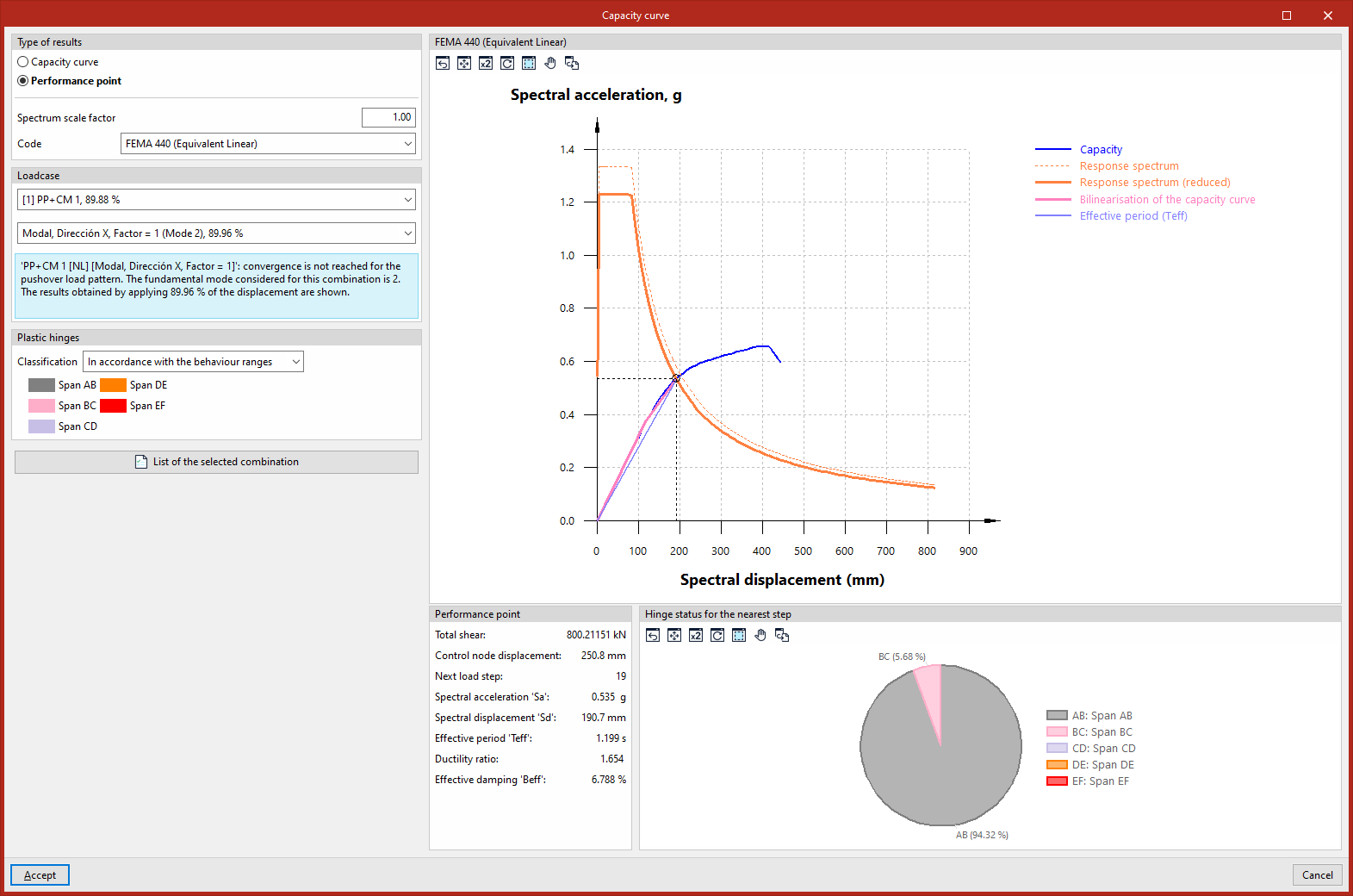
The program calculates the performance level based on the seismic code selected in the "General data" section. The methods implemented for the different codes are described in the following options. - FEMA 440 (Equivalent linearisation)
The program calculates the performance point using the Equivalent linearisation method (FEMA-440, 6.4 – Procedure A). This is a CSM (Capacity Spectrum Method). - ASCE 41-23
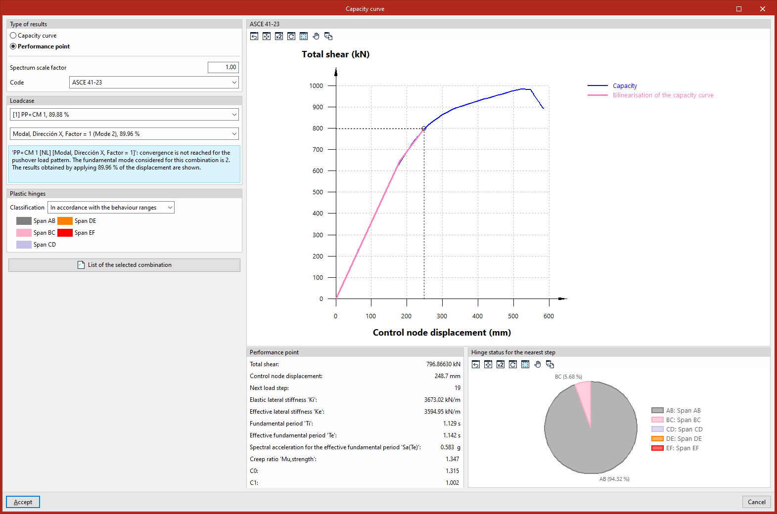
The program calculates the performance point using the Displacement Modification Method (ASCE 41-23, 7.4.3.3.2). This is a DCM (Displacement Control Method) - Eurocode 8-2004 (Target displacement)
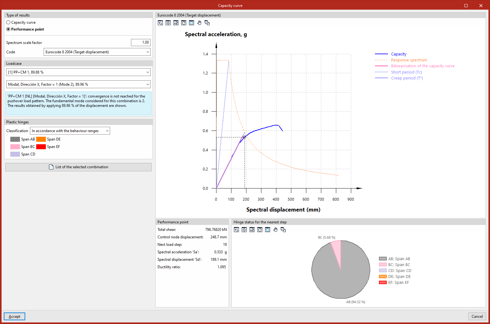
The program calculates the performance point using the N2 Method (Eurocode 8, Annex B). This is a CSM (Capacity Spectrum Method).
In addition, the program allows the user to adjust the "Spectrum scaling factor" as required.
Data query
Once a solution method has been selected, the graph on the right shows the "Spectral displacement (mm)" on the x-axis, whilst the y-axis shows the "Spectral acceleration, g", beneath which both the capacity curve and the elastic spectrum (defined in "General data", "With dynamic earthquake") are represented through a series of transformations.
The exact point at which a structure’s load-bearing capacity meets the seismic forces to which it is exposed represents the likely displacement the building will undergo during a specific earthquake.
The "Performance point" panel at the bottom displays data such as "Total Shear", "Control node displacement" and "Nearest load step".
The performance score obtained using the methods set out in the various standards should be reasonably similar.
Check the status of the plastic step covers for the nearest step
In the "Plastic hinges" panel on the left, you can define the "Classification" by selecting one of the following options:
- "According to the acceptance criteria" ("Immediate Occupancy (IO)", "Life Safety (LS)", "Collapse Prevention (CP)"),
- or "according to the performance zones" of the hinges ("Zone AB", "Zone BC", "Zone CD", "Zone DE", "Zone EF").
The "Hinge status for the nearest load step" panel, in the bottom right-hand corner, shows the percentage of hinges in each condition for the load step closest to the performance point.
Report
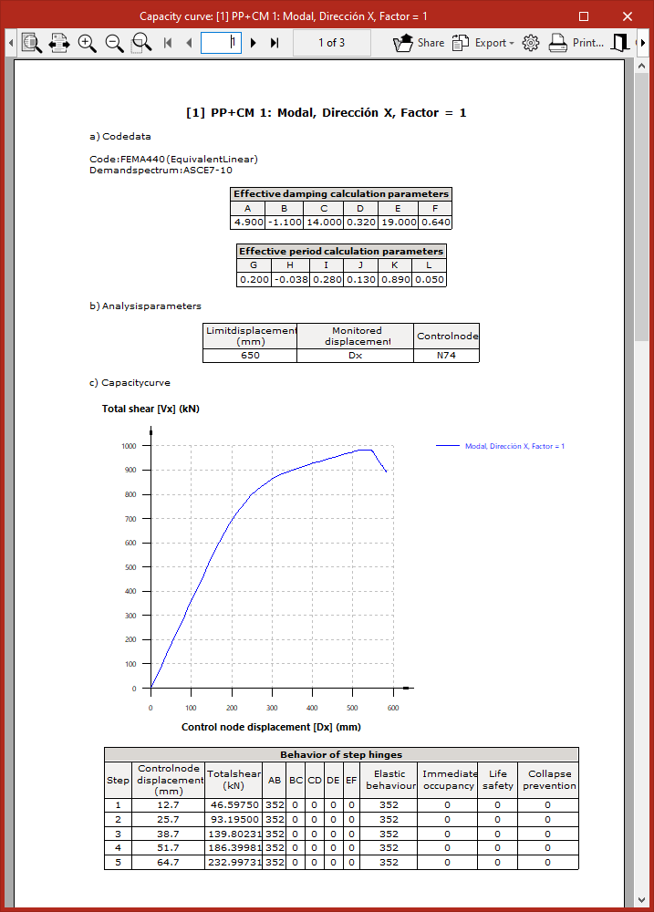
Finally, the program allows you to display on screen or print the "List of selected combinations" by clicking the relevant button in the "Capacity curve" window.
This report lists the data for the selected standard, the analysis parameters, the capacity curve, the step-by-step behaviour of the hinges, and the values associated with the performance point for the selected load case and standard.
Checking results for plastic hinges obtained from the pushover analysis
The results for plastic hinges obtained following the pushover analysis can be viewed using the "Plastic hinges" option, available in the "Pushover analysis" section of the top toolbar, within the "Analysis" tab (under the "Structure" tab):

Plastic hinges
Options in the "Properties-Selection" panel
Clicking on the "Plastic hinges" option opens the "Properties-Selection" window. Here, you must first select one of the following options:
- Bars
Displays the results for the plastic hinges defined in the selected bar. - Plastic hinges
Displays the individual results for the selected plastic hinge.
Load case
The results for the selected load case and lateral load pattern from the drop-down menus in the "Load case" panel on the left will be displayed.
On the label of the load case and/or load pattern, the fundamental mode considered is shown in brackets, whilst the percentage value indicates that the results shown have been obtained by applying that percentage of the target displacement.
In addition, in this panel you can select a specific level from the drop-down menu or navigate between levels using the various buttons provided.
This panel also displays a warning if convergence is not achieved for the selected load pattern.
If the target displacement is reached, the "Limit displacement" value is displayed, the "Monitored displacement" (Dx or Dy) is indicated, and the "Control node" reference is shown.
Plastic hinges
In the "Plastic hinges" panel on the left, you can define the "Classification" by selecting one of the following options:
- "In accordance with the acceptance criteria" ("Immediate occupancy (IO)", "Life safety (LS)", "Collapse prevention (CP)"); additionally, the hinge can be found under "Elastic behaviour (shown in grey);
- "In accordance with the performance zones" of the hinges ("Zone AB", "Zone BC", "Zone CD", "Zone DE", "Zone EF").
This way, the hinges will be represented as coloured spheres in the "Work area", scaled according to their state based on the defined classification and the selected load case, load pattern, and load step, thereby enabling the structure's behaviour to be analysed and potential failure mechanisms to be identified.
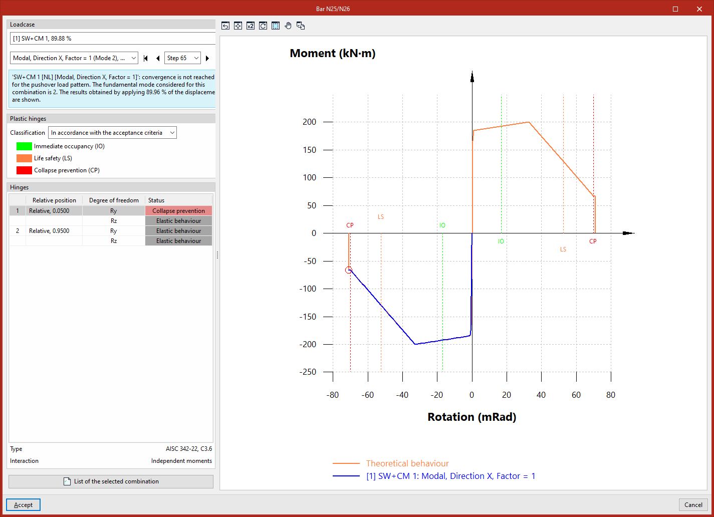
Checking the moment-rotation diagram for plastic hinges
When you click on a bar or a plastic hinge (depending on whether the "Bars" or "Plastic hinges" option has been selected in the "Properties-Selection" panel), the program will open a window allowing you to view the moment-rotation diagram (backbone curve) for the hinges assigned to the selected beam or the selected plastic hinge.
Here, you first select the load case, lateral pattern and step from the drop-down menus in the "Load case" panel on the left, in the same way as when viewing the other results of the pushover analysis.
In the "Plastic hinges" panel on the left, you can define the "Classification" as "According to acceptance criteria" or "According to the performance stages of the hinges". This will mark and label the different stages on the diagram using a dashed line.
The "Hinges" panel at the bottom lists the hinges that can be viewed in the window. For each entry in the list, the hinge number, its "Relative position" with respect to the bar, its "Degree of freedom", and its "Status" at the selected step and according to the previously selected classification are indicated. The bottom section displays the "Type" of each hinge and its "Interaction" ("Independent moments" or "Axil-My-Mz" interaction).
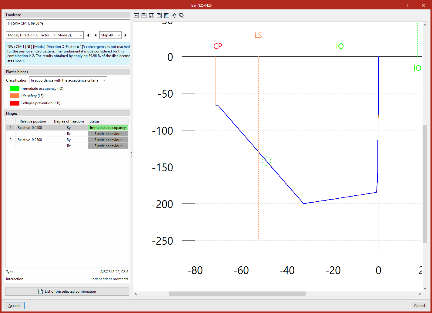
Moment-rotation diagram for plastic hinges with independent moments
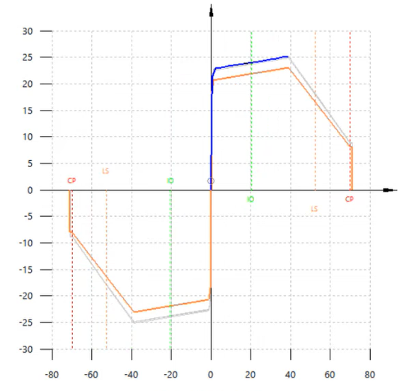
The graph shows the "Theoretical behaviour" of the selected ball-and-socket joint (at the selected degree of freedom) in orange, and the actual behaviour of the joint obtained from the pushover analysis performed by the software in blue.
A circle (coloured according to the condition of the hinge, using the same criteria as in the workspace)marks the exact point on the actual performance curve where the hinge is located at the selected step. Thus, by navigating between different steps, you can observe the movement of the circle along the actual performance curve.
Moment-rotation diagram for plastic hinges with axial-moment-moment interaction
In the "Axil-My-Mz" interaction hinges, the "Theoretical behaviour" curve is different for each step. However, the hinge’s operating point (represented by the circle shown) always lies on both the actual performance curve (in blue) and the theoretical performance curve for the selected stage (in orange). This curve is scaled by the value of the axil.
The remaining theoretical performance curves associated with the unselected steps are shown in light grey.
Report
Finally, the program allows you to display on screen or print the "List of selected combinations" by clicking on the relevant button in the plastic hinge query window.
This report lists the data for the selected standard, the analysis parameters, and the moment-rotation diagram for each hinge and selected degree of freedom, including the "Hinge properties" and a numerical table showing the "Results per step".
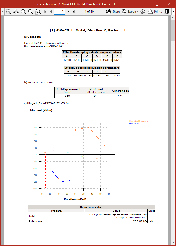
Table of contents
Complete your CYPE 3D journey by exploring the other available sections:
- Introduction
- Start: creating new projects, workflows, and examples
- Setting the work environment
- Setting the job data
- Defining the structure’s geometry
- Editing the properties of structural elements
- Entering and editing loads on the structure
- Designing and analysing connections
- Analyses, checks, and results
- Defining and editing reinforcement
- Designing and analysing foundation
- Printing documents and exporting data